Signaling Network Reconstruction Using Bayesian Networks In R
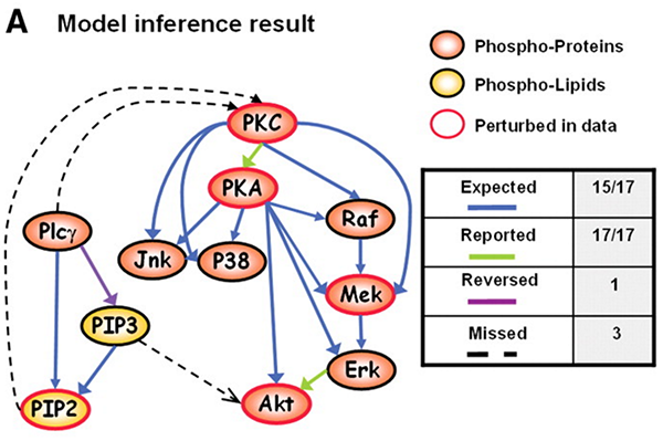
In in landmark paper “Causal Protein-Signaling Networks Derived from Multiparameter Single-Cell Data”, Sachs et al. applied Bayesian Networks on multi-parameter flow cytometry data to reconstruct signaling relationships and predict novel interpathway network causalities. Following a tutorial by Marco Scutari, I attempt to reproduce to the best of my abilities the statistical analysis of the paper using Marco’s bnlearn R package.
library(bnlearn)
library(Rgraphviz)
First, read in and process the data. Since this is flow cytometry data, it must be transformed to make the data look more normal and biologically interpretable.
sachs = read.table("data/sachs.data.txt", header = TRUE)
sachs <- as.matrix(sachs)
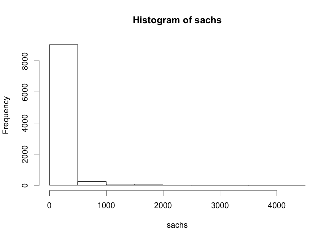
## assess distribution of data
hist(sachs)
## standard transformation for flow cytometry data
sachs <- asinh(sachs)

## assess distribution of data
hist(sachs)
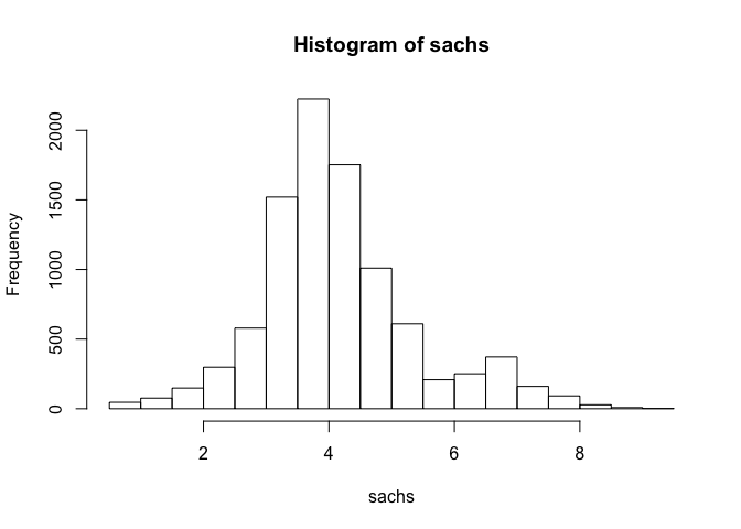
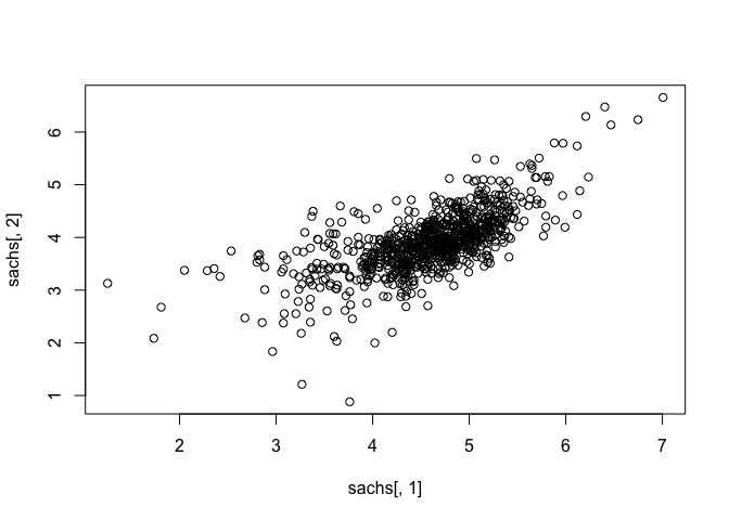
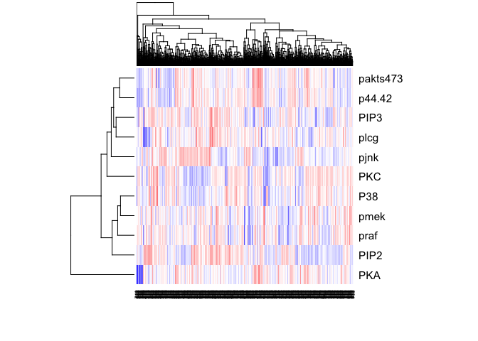
Note that the data appears normally distributed with no obvious zero-inflation or otherwise missing data, suggesting good quality. We can already readily see correlation structures within the data.
## assess correlations
plot(sachs[, 1], sachs[,2])
heatmap(t(as.matrix(sachs)), col=colorRampPalette(c("blue", "white", "red"))(100), scale="row")
sachs <- data.frame(sachs)
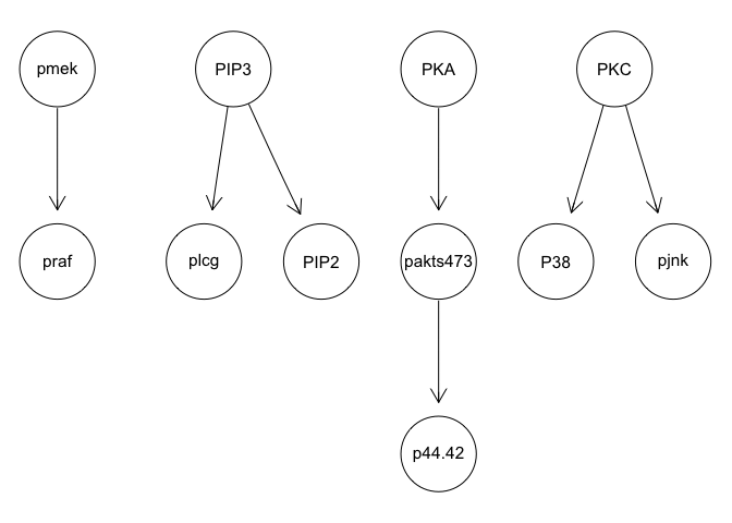
We can run some simple Bayesian network structure inferences. However, these results are highly unstable and do not recapitulate the known network structure.
g <- inter.iamb(sachs, test = "smc-cor", B = 500, alpha = 0.01)
graphviz.plot(g)
g <- hc(sachs, score = "bge", iss = 3, restart = 5, perturb = 10)
graphviz.plot(g)
g <- tabu(sachs, tabu = 50)
graphviz.plot(g)
g <- mmhc(sachs)
graphviz.plot(g)
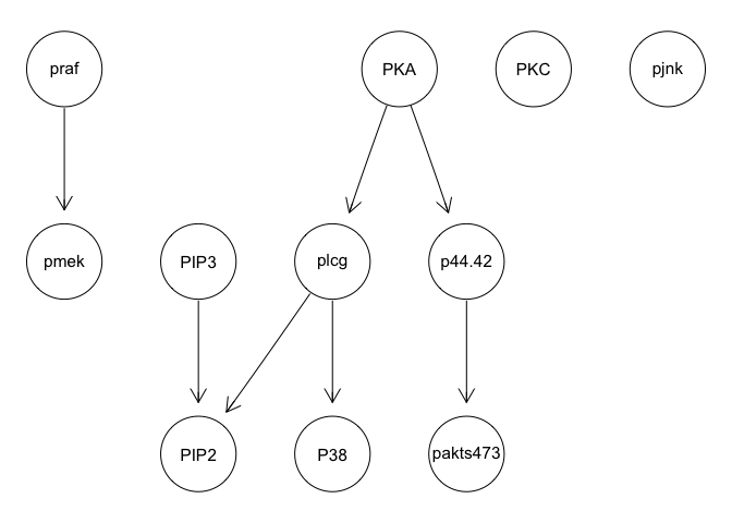
We can apply various techniques such as discretization and model averaging to improve stability. However, results still poorly recapitulate the known network structure.
## discritize
dsachs = discretize(sachs, method = "hartemink", breaks = 3, ibreaks = 60, idisc = "quantile")
## model average
boot = boot.strength(data = dsachs, R = 500, algorithm = "tabu", algorithm.args=list(tabu = 50))
boot[(boot$strength >= 0.85) & (boot$direction >= 0.5), ]
##from   to strength direction
## 1  praf pmek1.000 0.5000000
## 11 pmek praf1.000 0.5000000
## 23 plcg PIP20.994 0.5080483
## 24 plcg PIP30.982 0.5020367
## 44 PIP3 PIP21.000 0.5060000
## 56   p44.42 pakts4731.000 0.5000000
## 66 pakts473   p44.421.000 0.5000000
## 67 pakts473  PKA0.996 0.5000000
## 77  PKA pakts4730.996 0.5000000
## 89  PKC  P381.000 0.5010000
## 90  PKC pjnk1.000 0.5060000
plot(boot)
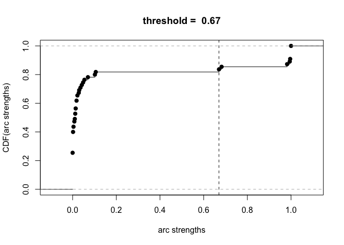
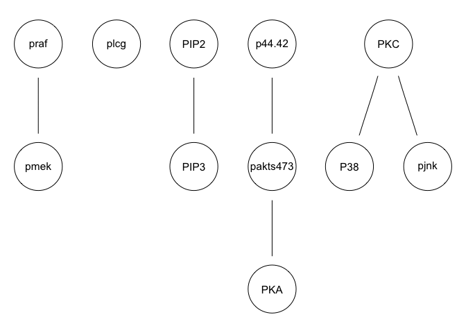
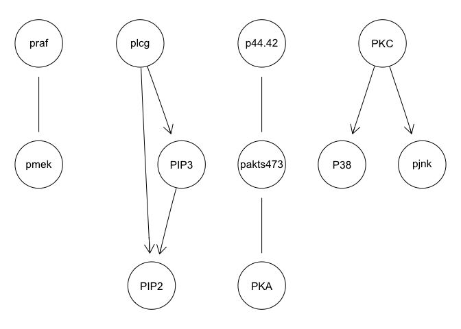
avg.boot = averaged.network(boot, threshold = 0.85)
graphviz.plot(avg.boot)
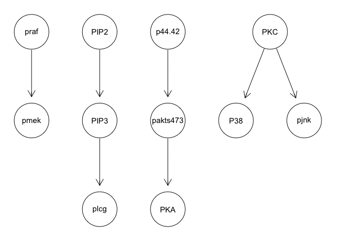
The original paper suggests that network interventions are needed for accurate inference. So let’s use the interventional data. The values of INT identifies which node is subject to either a stimulatory cue or an inhibitory intervention. Note that such data requires some degree of prior knowledge about pathway relationships, which may not always be available.
## interventions
isachs = read.table("data/sachs.interventional.txt", header = TRUE, colClasses = "factor")
INT = sapply(1:11, function(x) { which(isachs$INT == x) })
isachs = isachs[, 1:11]
## factor data
head(isachs)
##   praf pmek plcg PIP2 PIP3 p44.42 pakts473 PKA PKC P38 pjnk
## 111123  21   3   1   21
## 211113  32   3   1   21
## 311223  21   3   2   11
## 411113  21   3   1   31
## 511113  21   3   1   11
## 611112  21   3   1   21
nodes = names(isachs)
names(INT) = nodes
start = random.graph(nodes = nodes, method = "melancon", num = 500, burn.in = 10^5, every = 100)
netlist = lapply(start, function(net) {
tabu(isachs, score = "mbde", exp = INT, iss = 1, start = net, tabu = 50)
})
arcs = custom.strength(netlist, nodes = nodes, cpdag = FALSE)
bn.mbde = averaged.network(arcs, threshold = 0.85)
graphviz.plot(bn.mbde)
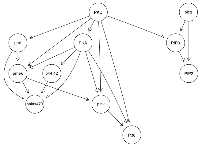
bn.mbde
##
##   Random/Generated Bayesian network
##
##   model:
##[plcg][PKC][praf|PKC][PIP3|plcg:PKC][PKA|PKC][pmek|praf:PKA:PKC]
##[PIP2|plcg:PIP3][p44.42|PKA][pakts473|praf:pmek:p44.42:PKA]
##[pjnk|pmek:PKA:PKC][P38|PKA:PKC:pjnk]
##   nodes: 11
##   arcs:  20
## undirected arcs: 0
## directed arcs:   20
##   average markov blanket size:   4.36
##   average neighbourhood size:3.64
##   average branching factor:  1.82
##
##   generation algorithm:  Model Averaging
##   significance threshold:0.85
As you can see, with the interventional data, we are generally able to
recapitulate the published results.
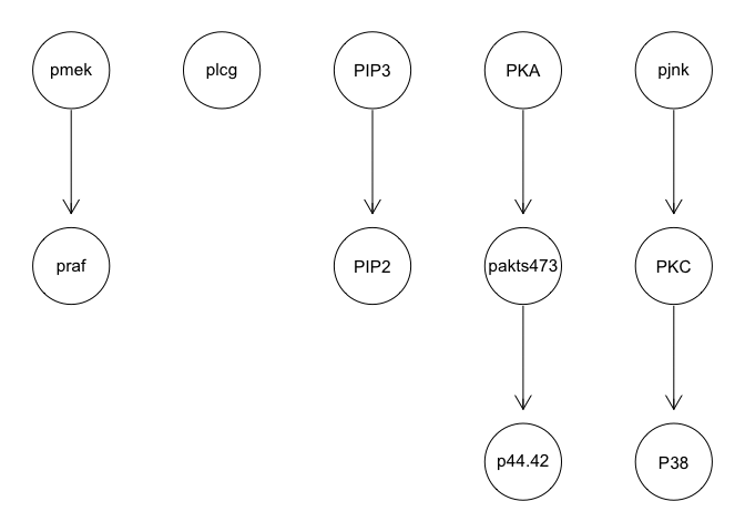
The original paper also suggested that the large number of cells was necessary for accurate network reconstruction. So what happens if we subsample to a smaller number of cells?
isachs = read.table("data/sachs.interventional.txt", header = TRUE, colClasses = "factor")
dim(isachs)
## [1] 5400 12
## subsample 50 cells from each intervention
isachs <- do.call(rbind, lapply(seq_len(length(levels(isachs$INT))), function(i) {
  d <- isachs[as.numeric(isachs$INT)==i, ]
  if(nrow(d) > 50) {
return (d[1:50,])
  }
}))
dim(isachs)
## [1] 300 12
INT = sapply(1:11, function(x) { which(isachs$INT == x) })
isachs = isachs[, 1:11]
nodes = names(isachs)
names(INT) = nodes
start = random.graph(nodes = nodes, method = "melancon", num = 500, burn.in = 10^5, every = 100)
netlist = lapply(start, function(net) {
tabu(isachs, score = "mbde", exp = INT, iss = 1, start = net, tabu = 50)
})
arcs = custom.strength(netlist, nodes = nodes, cpdag = FALSE)
bn.mbde = averaged.network(arcs, threshold = 0.85)
graphviz.plot(bn.mbde)
As expected, results poorly recapitulate known network structure. Thus, consistent with the paper findings, a large number of cells and inclusion of interventional data is needed for accurate network reconstruction.
Recent Posts
- AI-guided data visualization of gas prices in different geographical locations across the US over time on 04 May 2026
- The Mentorship Index on 01 March 2026
- Vibe coding with SEraster and STcompare to compare spatial transcriptomics technologies on 22 February 2026
- RNA velocity in situ infers gene expression dynamics using spatial transcriptomics data on 13 October 2025
- Analyzing ICE Arrest Data - Part 2 on 27 September 2025