Bioinformatics for custom sequencing library constructions

Sequencing has become so streamlined that we often just use standard library prep kits, made for particular sequencers, followed by proprietary bioinformatics software for demultiplexing and quantification. But, if we want to design custom library structure, perhaps for use in multiplexed droplet-based approaches, we will need to come up with our own bioinformatics pipelines. In this tutorial, I will take you through a recent experience I had analyzing reads from a custom library prep.

Consider the library structure below:

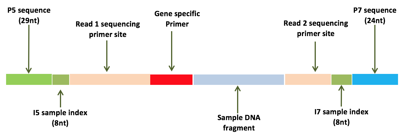
For this particular library, we’ve used custom gene specific primers for targeted sequencing of specific genes containing mutations of interest (as opposed to doing a whole exome for example). Let’s assume the data has already been demultiplexed and the paired-end reads have been properly split. Thus, what we should have in our FASTQs are a bunch of sequences containing the gene specific primers and our sample DNA fragment of interest.

For simplicity, let’s just look at one forward read.

library(ShortRead)
file1 <- "../data-raw/N706_S1_L001_R1_001.fastq.gz"  
fastq1 <- readFastq(file1)
r1trim <- fastq1@sread[1] 
as.character(r1trim)

GGAAGCTGCAGCCCTCACTTAACAGTGGGCGGCTCCTCCATCTAGCCATGCGAGGTCTTGGGGAGCTGGGCGCCCAGCCCCAACAGGACCATGCACGCTGGCCCCGGGGCAGCAGCCTGTCCGAGTGCA

Our first goal is to figure out which gene specific primer is being used for this read. Since we know the sequences for all our gene specific primers, we can just try to align each to our read. Because of potential sequencing errors in the primer itself and since each primer may be a different length, using a simple Needleman–Wunsch alignment algorithm will likely save more reads than just simple string matching.

## primers.valid is a DNAStringSet containing our primer sequences
## so we can assess how well each primer matches our sequence
scores <- sapply(1:length(primers.valid), function(j) {    
   p <- primers.valid[j]       
   r <- DNAStringSet(substring(as.character(r1trim), 0, width(p)))  
   mat <- nucleotideSubstitutionMatrix(match = 100, mismatch = -1, baseOnly = TRUE)     
   align <- pairwiseAlignment(p, r, substitutionMatrix = mat, gapOpening = -1, gapExtension = -1) 
   ## divide by theoretical max
   score(align)/(width(p)*100) 
}) 
j <- which(scores==max(scores)) ## the theoretical max should be 1
p <- primers.valid[j] ## DNAString of the sequence
pr <- primers.valid.info[j,] ## information about the primer
pr

       chr     pos strand width   start     end  width seq       
 397 chr17 9792856      +    26 9792832 9792857     26 GGAAGCTGCAGCCCTCACTTAACAGT

So let’s look more closely at the gene specific primer that this sequence matched with. Indeed, we can visually/manually confirm that this is the correct primer:

GGAAGCTGCAGCCCTCACTTAACAGTGGGCGGCTCCTCCATCTAGCCATGCGAGGTCTTGGGGAGCTGGGCGCCCAGCCCCAACAGGACCATGCACGCTGGCCCCGGGGCAGCAGCCTGTCCGAGTGCA
GGAAGCTGCAGCCCTCACTTAACAGT

Or just quickly realign to double check.

r <- DNAStringSet(substring(as.character(r1trim), 0, width(p)))   
mat <- nucleotideSubstitutionMatrix(match = 100, mismatch = -1, baseOnly = TRUE)      
align <- pairwiseAlignment(p, r, substitutionMatrix = mat, gapOpening = -1, gapExtension = -1)  
align

 Global PairwiseAlignmentsSingleSubject (1 of 1)     
 pattern: [1] GGAAGCTGCAGCCCTCACTTAACAGT   
 subject: [1] GGAAGCTGCAGCCCTCACTTAACAGT   
 score: 2600 

Yay it’s a perfect match! And we can trim off this gene specific primer to get just the target DNA sequence.

r1final <- DNAStringSet(substring(as.character(r1trim), width(p)+1))
as.character(r1final)

GGGCGGCTCCTCCATCTAGCCATGCGAGGTCTTGGGGAGCTGGGCGCCCAGCCCCAACAGGACCATGCACGCTGGCCCCGGGGCAGCAGCCTGTCCGAGTGCA

Hurray! But now we need to align it to the reference genome. We could take these trimmed reads and run an aligner, but since we know where our gene specific primer is located, we can just look at the upstream or downstream DNA sequence. Note, depending on the strand of the primer (forward vs. reverse), the start and end positions of the DNA sequence that will be sequenced will be different. And always double check for those off-by-one errors!

if(pr$strand=='+') {  
    start=pr$end+1      
    end=pr$end+width(r1final) 
} 
if(pr$strand=='-') {  
    start=pr$start-width(r1final)+1    
    end=pr$start      
}
align.df <- data.frame(chr=pr$chr, strand=pr$strand, start=start, end=end)
library(GenomicRanges)  
align.gr <- with(align.df, GRanges(chr, IRanges(as.numeric(start), as.numeric(end)), strand=strand)) 
library(BSgenome.Hsapiens.UCSC.hg19)         
align.seq <- getSeq(BSgenome.Hsapiens.UCSC.hg19, align.gr)       
as.character(align.seq)        

GGGCGGCTCCTACATCTAGCCATGCGAGGTCTTGGGGAGCTGGGCGCCCAGCCCCAACAGGACCATGCACGCTGGCCCCGGGGCAGCAGCCTGTCCGAGTGCA

Visually/manually checking how well our sequenced read (top) matches the reference (bottom), we see a very good match!

GGGCGGCTCCTCCATCTAGCCATGCGAGGTCTTGGGGAGCTGGGCGCCCAGCCCCAACAGGACCATGCACGCTGGCCCCGGGGCAGCAGCCTGTCCGAGTGCA
GGGCGGCTCCTACATCTAGCCATGCGAGGTCTTGGGGAGCTGGGCGCCCAGCCCCAACAGGACCATGCACGCTGGCCCCGGGGCAGCAGCCTGTCCGAGTGCA

Now we can find mutation using simple string comparison.

ref <- strsplit(as.character(align.seq), split="")[[1]]
read <- strsplit(as.character(r1final), split="")[[1]]
muts <- do.call(rbind, lapply(1:length(ref), function(i) {       
    if(ref[i]!=read[i]) {   
        s = pr$strand       
        if(s=='+'){         
            r = ref[i]      
            m = read[i]     
        } else {  
            r = as.character(complement(DNAString(ref[i])))      
            m = as.character(complement(DNAString(read[i])))     
        }         
        info <- data.frame('chr'=pr$chr, 'pos'=start+i-1, 'strand'='+', 'ref'=r, 'mut'=m)        
        return(info)        
    }   
}))
muts

     chr     pos strand ref mut     
 1 chr17 9792869      +   A   C

Final double check that that our position is correct.

align.df <- data.frame(chr=muts$chr, strand=muts$start, start=muts$pos, end=muts$pos) 
align.gr <- with(align.df, GRanges(chr, IRanges(as.numeric(start), as.numeric(end)), strand=strand)) 
align.seq <- getSeq(BSgenome.Hsapiens.UCSC.hg19, align.gr)
align.seq

A DNAStringSet instance of length 1 
    width seq
[1]     1 A

Since this could be a sequencing error, we can rely on other information such as the read quality or just look at other reads to see if this mutation pops up again. As you can already tell, things become a little more complicated for reverse primer reads since we need to get complements. Similarly for reverse reads, we need to get reverse complement sequences, which can quickly become confusing if you don’t double check your work by comparing to references and keeping track of the directionality!