Graph-based community detection for clustering analysis in R

Introduction

In single cell analyses, we are often trying to identify groups of transcriptionally similar cells, which we may interpret as distinct cell types or cell states. We may also be interested in identifying groups of transcriptionally coordinated genes, which we may interpret as functional regulatory modules or pathways. In either case, we are looking at some high dimensional data and trying to identify clusters.

We can also think of these clusters as communities in a graph. Abstractly, our graph would just be composed of all our cells as vertices. And the vertices would, in theory, be connected to each other if the cells were of the same cell type. Community detection in graphs identify groups of vertices with higher probability of being connected to each other than to members of other groups.

In this tutorial, I will use simulated and public data to demonstrate how you can apply graph-based community detection to identify cell types.

Simulation

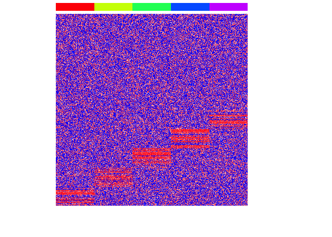
First, let’s simulate some data. We will simulate 5 very clearly distinct cell types and see if we can use graph-based community detection to correctly recover the true cell type annotations.

G=5 ## number of cell types
N=100 ## number of cells per cell type
M=1000 ## number of genes
initmean=0 ## baseline mean expression
initvar=10 ## baseline expression variance
upreg=10 ## degree of cell-type specific upregulation
upregvar=10 ## expression variance of upregulated genes
ng=100 ## number of upregulated genes per cell type
seed=0 ## random seed

set.seed(seed)
mat <- matrix(rnorm(N*M*G, initmean, initvar), M, N*G)
rownames(mat) <- paste0('gene', 1:M)
colnames(mat) <- paste0('cell', 1:(N*G))
group <- factor(sapply(1:G, function(x) rep(paste0('group', x), N)))
names(group) <- colnames(mat)

diff <- lapply(1:G, function(x) {
    diff <- rownames(mat)[(((x-1)*ng)+1):(((x-1)*ng)+ng)]
    mat[diff, group==paste0('group', x)] <<- mat[diff, group==paste0('group', x)] + rnorm(ng, upreg, upregvar)
    return(diff)
})
names(diff) <- paste0('group', 1:G)

mat[mat<0] <- 0
mat <- t(t(mat)/colSums(mat))
mat <- log10(mat*1e6+1)

heatmap(mat, Rowv=NA, Colv=NA, col=colorRampPalette(c('blue', 'white', 'red'))(100), scale="none", ColSideColors=rainbow(G)[group], labCol=FALSE, labRow=FALSE)

To apply graph-based community detection algorithms, we will need to represent our data as a graph. To do this, we will use the RANN to identify approximate nearest neighbors.

library(RANN)
knn.info <- RANN::nn2(t(mat), k=30)

The result is a list containing a matrix of neighbor relations and another matrix of distances. We will convert this neighbor relation matrix into an adjacency matrix.

knn <- knn.info$nn.idx
adj <- matrix(0, ncol(mat), ncol(mat))
rownames(adj) <- colnames(adj) <- colnames(mat)
for(i in seq_len(ncol(mat))) {
    adj[i,colnames(mat)[knn[i,]]] <- 1
}

Now, we can represent the adjacancy matrix as a graph.

library(igraph)
g <- igraph::graph.adjacency(adj, mode="undirected")
g <- simplify(g) ## remove self loops
V(g)$color <- rainbow(G)[group[names(V(g))]] ## color nodes by group
plot(g, vertex.label=NA)

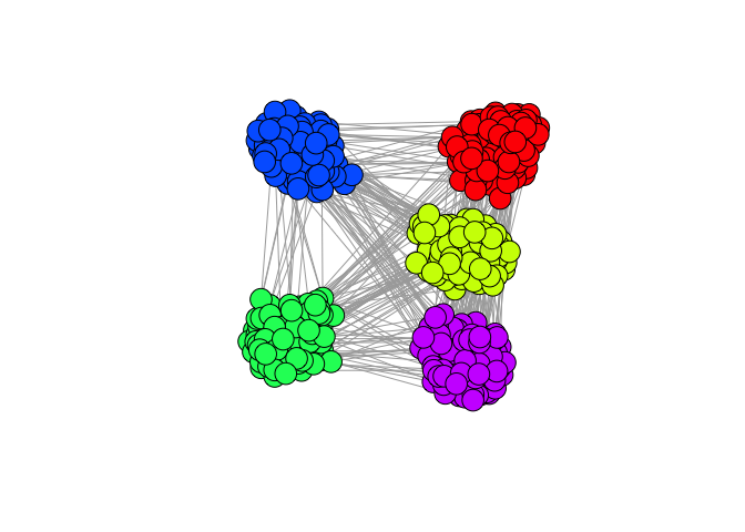
In visualizing the graph, we can clearly see 5 very distinct communities corresponding to our simulated cell types. If we can see these distinct communities, surely a graph-based community detection method such as the walktrap algorithm can detect them too.

km <- igraph::cluster_walktrap(g)
## community membership
com <- km$membership
names(com) <- km$names
table(com, group)

##    group
## com group1 group2 group3 group4 group5
##   1    100      0      0      0      0
##   2      0    100      0      0      0
##   3      0      0      0      0    100
##   4      0      0      0    100      0
##   5      0      0    100      0      0

Do our identified communities match our simulated groups? Indeed they do! Community 1 corresponds to our group1 of cells, community 2 to our group2, community 3 to our group5, and so forth. However, this is a perfect simulated world. What happens when we apply this to real world data?

10X Immune Cells

Consider this public dataset from 10X genomics.

library(Matrix)
load('reference_10x.RData')
dim(reference.cd)

## [1] 32738  2140

table(ct)

## ct
##         bcells     cytotoxict        memoryt      monocytes naivecytotoxic 
##            330            148            252            129             43 
##         naivet             nk    regulatoryt        thelper 
##             52            769            226            191

Let’s clean up this data a little. We’ll remove genes seen in fewer than 100 cells (a bit stringent, but it’ll speed things up for this demonstration). Then we’ll normalize and log transform.

vi <- Matrix::rowSums(reference.cd>0)>100
table(vi)

## vi
## FALSE  TRUE 
## 27704  5034

mat <- reference.cd[vi,]
mat <- t(t(mat)/colSums(mat))
mat <- log10(mat*1e6+1)
mat[1:5,1:5]

## 5 x 5 Matrix of class "dgeMatrix"
##          bcellsAAAGATCTCCGAAT-1 bcellsAAAGCAGAGTACGT-1
## NOC2L                   0.00000                      0
## ISG15                   2.43014                      0
## TNFRSF18                2.43014                      0
## TNFRSF4                 0.00000                      0
## SDF4                    0.00000                      0
##          bcellsAAATCTGACCCTTG-1 bcellsAACAGCACTGAACC-1
## NOC2L                  0.000000               0.000000
## ISG15                  2.461924               2.432584
## TNFRSF18               0.000000               2.432584
## TNFRSF4                0.000000               0.000000
## SDF4                   2.461924               2.432584
##          bcellsAACATTGATGCTTT-1
## NOC2L                  2.799293
## ISG15                  3.099978
## TNFRSF18               0.000000
## TNFRSF4                0.000000
## SDF4                   0.000000

Now let’s run our graph-based community detection to see if we recover the true cell type annotations.

## identify KNN
library(RANN)
knn.info <- RANN::nn2(t(mat), k=30)

## convert to adjacancy matrix
knn <- knn.info$nn.idx
adj <- matrix(0, ncol(mat), ncol(mat))
rownames(adj) <- colnames(adj) <- colnames(mat)
for(i in seq_len(ncol(mat))) {
    adj[i,colnames(mat)[knn[i,]]] <- 1
}

## convert to graph
library(igraph)
g <- igraph::graph.adjacency(adj, mode="undirected")
g <- simplify(g) ## remove self loops

## identify communities
km <- igraph::cluster_walktrap(g)
com <- km$membership
names(com) <- km$names

## compare to annotations
table(com, ct)

##    ct
## com bcells cytotoxict memoryt monocytes naivecytotoxic naivet  nk
##   1      0          5      20         1              0      1   0
##   2      0          0       1       110              0      2   0
##   3    330          0       0        17              1      6   0
##   4      0        137     231         1             42     43   3
##   5      0          6       0         0              0      0 766
##    ct
## com regulatoryt thelper
##   1          16      15
##   2           3       8
##   3           0       0
##   4         207     168
##   5           0       0

Not perfect but not bad! Community 3 is predominantly b cells, community 4 is cytotoxic t cells, community 2 is monocytes, and so forth. There are lots of other community detection algorithms as well that we can try like infomap.

km <- igraph::cluster_infomap(g)
com <- km$membership
names(com) <- km$names
table(com, ct)

##    ct
## com bcells cytotoxict memoryt monocytes naivecytotoxic naivet  nk
##   1      0        140     217         0             42     34   3
##   2      0          3       0         0              0      0 766
##   3    330          0       0         2              0      0   0
##   4      0          0       1       110              0      2   0
##   5      0          5      20         0              0      0   0
##   6      0          0      14         0              0      9   0
##   7      0          0       0        17              1      7   0
##    ct
## com regulatoryt thelper
##   1         208     165
##   2           0       0
##   3           0       0
##   4           3       8
##   5          14      13
##   6           1       4
##   7           0       1

And many many more. Check out the igraph package for more community detection algorithms available through the package: https://www.rdocumentation.org/packages/igraph/

Now it’s time for you to try it out for yourself. What if we change k in the k-nearest neighbor identification? What if we use fewer features/genes? What if we try a different community detection algorithm? What if we transpose our matrices and try to cluster genes instead of cells?