Machine Learning Feature Selection For Diffexp Analysis
Feature Selection for Differential Expression Analysis and Marker Selection
Introduction
In transcriptomics analysis, we are often interested in identifying differentially expressed genes. For example, if we have two conditions or cell types, we may be interested in what genes are significantly upregulated in condition A vs. B or cell type X vs. Y and vice versa. Differential expression analysis is often performed as Wilcox tests, T-tests, or other similar tests for differences in distribution.
However, in many situations, such as in selecting marker genes for downstream validation of a potentially new cell subpopulation or in cell sorting, we not only want to identify genes that are differentially expressed in this subpopulation versus all other cell types, but we also want genes that, potentially in combiation, mark just this subpopulation and not any other cell type. So this starts to sound like a machine learning feature selection problem: what genes or features can be used to train a machine learning classifier to identify this subpopulation of cells?
In this tutorial, I will build upon my previous blog post on Multi-class / Multi-group Differential Expression Analysis, using simulated data to demonstrate potential machine learning approaches to identify differentially expressed candidate marker genes.
Simulation
First, let’s simulate some data. This is the basically the same simulated data as in Multi-class / Multi-group Differential Expression Analysis except I’ve modified 2 genes so that they will in combination identify cells in group1.
set.seed(0)
G <- 5
N <- 30
M <- 1000
initmean <- 5
initvar <- 10
mat <- matrix(rnorm(N*M*G, initmean, initvar), M, N*G)
rownames(mat) <- paste0('gene', 1:M)
colnames(mat) <- paste0('cell', 1:(N*G))
group <- factor(sapply(1:G, function(x) rep(paste0('group', x), N)))
names(group) <- colnames(mat)
set.seed(0)
upreg <- 5
upregvar <- 10
ng <- 100
diff <- lapply(1:G, function(x) {
diff <- rownames(mat)[(((x-1)*ng)+1):(((x-1)*ng)+ng)]
mat[diff, group==paste0('group', x)] <<- mat[diff, group==paste0('group', x)] + rnorm(ng, upreg, upregvar)
return(diff)
})
names(diff) <- paste0('group', 1:G)
diff2 <- lapply(2:(G-1), function(x) {
y <- x+G
diff <- rownames(mat)[(((y-1)*ng)+1):(((y-1)*ng)+ng)]
mat[diff, group %in% paste0("group", 1:x)] <<- mat[diff, group %in% paste0("group", 1:x)] + rnorm(ng, upreg, upregvar)
return(diff)
})
## remove negative values in this simulation to be more like real gene expression data
mat[mat<0] <- 0
## add in fake perfect FACs markers
ct <- "group1"
markers.true <- as.numeric(group==ct)
set.seed(0)
vi1 <- sample(which(markers.true==1), 5)
vi2 <- sample(setdiff(which(markers.true==1), vi1), 5)
markers1 <- markers2 <- markers.true + 0.1
markers1[vi1] <- 0
markers2[vi2] <- 0
mat[1,] <- mat[1,]*markers1
mat[10,] <- mat[10,]*markers2
## so true FACs genes for group1 should be 1 and 10
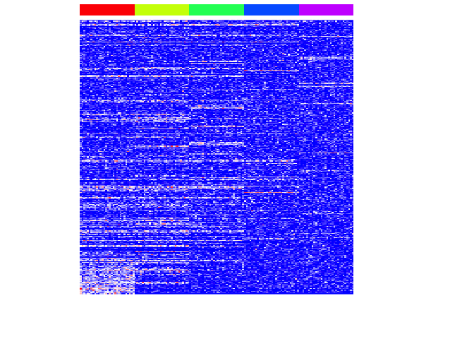
heatmap(mat, Rowv=NA, Colv=NA, col=colorRampPalette(c('blue', 'white', 'red'))(100), scale="none", ColSideColors=rainbow(G)[group], labCol=FALSE, labRow=FALSE)

Machine learning with mlr
The mlr (Machine Learning in R) package very nicely pulls in machine learning approaches from other packages into a single integrated framework for machine learning experiments in R. They also have lots of great tutorials to help you get started](https://mlr-org.github.io/mlr-tutorial/release/html/index.html).
First, we can define a classification task as classify cells as group1.
library(mlr)

## Create data frame with data
ct <- "group1"
mat.test <- as.data.frame(t(mat))
mat.test$celltype <- group[rownames(mat.test)]==ct
## Define the task
## Specify the type of analysis (e.g. classification) and provide data and response variable
task <- makeClassifTask(data = mat.test, target = "celltype")
We will use mlr’s function generateFilterValuesData to perform feature selection. A table showing all available feature selection methods can be found here.
I will select features based on their importance in a random forest classifier. Feature selection based on a decision tree-based approach such as with a random forest classifier makes sense intuitively if we wanted to find a set of potential surface markers for FACs and had a matrix of gene expression for cell surface protein encoding genes. We want to build a decision tree or group of decision trees that will tell if that us if we gate cells on expression of X and then Y, we will get our population of interest.
method <- 'cforest.importance'
fv <- generateFilterValuesData(task, method = method)
results <- fv$data
results <- results[order(results[,3], decreasing=TRUE),]
head(results)
##      name    type cforest.importance
## 1   gene1 numeric        0.004763636
## 3   gene3 numeric        0.003745455
## 4   gene4 numeric        0.003418182
## 98 gene98 numeric        0.003272727
## 91 gene91 numeric        0.003200000
## 10 gene10 numeric        0.003054545
We can filter for genes with non-zero importance and visualize the results.
t <- 0
pv.sig <- na.omit(results$name[results[,3]>t])
heatmap(mat[pv.sig,], Rowv=NA, Colv=NA, col=colorRampPalette(c('blue', 'white', 'red'))(100), scale="none", ColSideColors=rainbow(G)[group], labCol=FALSE, labRow=FALSE)
Now let’s repeat this for each subpopulation.
t <- 0
method <- 'cforest.importance'
pv.sig <- lapply(levels(group), function(ct) {
mat.test <- as.data.frame(as.matrix(t(mat)))
mat.test$celltype <- group[rownames(mat.test)]==ct
task <- makeClassifTask(data = mat.test, target = "celltype")
fv <- generateFilterValuesData(task, method = method)
results <- fv$data
results <- results[order(results[,3], decreasing=TRUE),]
pv.sig <- na.omit(results$name[results[,3]>t])
})
names(pv.sig) <- levels(group)
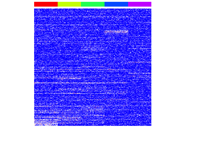
heatmap(mat[unique(unlist(pv.sig)),], Rowv=NA, Colv=NA, col=colorRampPalette(c('blue', 'white', 'red'))(100), scale="none", ColSideColors=rainbow(G)[group], labCol=FALSE, labRow=FALSE)
We can assess our performance by comparing our identified important genes to those we simulated as important.
perf <- function(pv.sig) {
    predtrue <- unique(unlist(pv.sig)) ## predicted differentially expressed genes
    predfalse <- setdiff(rownames(mat), predtrue) ## predicted not differentially expressed genes
    true <- c(unlist(diff), unlist(diff2)) ## true differentially expressed genes
    false <- setdiff(rownames(mat), true) ## true not differentially expressed genes
    TP <- sum(predtrue %in% true)
    TN <- sum(predfalse %in% false)
    FP <- sum(predtrue %in% false)
    FN <- sum(predfalse %in% true)
    sens <- TP/(TP+FN)
    spec <- TN/(TN+FP)
    prec <- TP/(TP+FP)
    fdr <- FP/(TP+FP)
    acc <- (TP+TN)/(TP+FP+FN+TN)
    return(data.frame(sens, spec, prec, fdr, acc))
}
print(perf(pv.sig))
##     sens  spec      prec       fdr   acc
## 1 0.8475 0.385 0.8464419 0.1535581 0.755
Looks like we did pretty well!
But let’s get back to our FACs problem and say we really want to identify just 2 markers that will help us sort out group1 cells from all others. Let’s calculate the 10-fold cross-validated error rate of simple decision tree classifier (classif.rpart) with preceding feature selection. We will again use cforest.importance as importance measure and select the 2 features with highest importance. We can then look at which features were consistently selected in our cross-validations
ct <- "group1"
mat.test <- as.data.frame(t(mat))
mat.test$celltype <- group[rownames(mat.test)]==ct
task <- makeClassifTask(data = mat.test, target = "celltype")

## fuse learner with feature selection
lrn <- makeFilterWrapper(learner = "classif.rpart", fw.method = "cforest.importance", fw.abs = 2) ## 2 features only
rdesc <- makeResampleDesc("CV", iters = 10)
r <- resample(learner = lrn, task = task, resampling = rdesc, show.info = FALSE, models = TRUE)

## get features used
sfeats <- sapply(r$models, getFilteredFeatures)
markers <- sort(table(sfeats), decreasing=TRUE)
print(markers)
## sfeats
##  gene10   gene1   gene3  gene91  gene98  gene39  gene41  gene48 gene699
##       6       4       2       2       2       1       1       1       1
## take best 2 across CVs
marker <- names(markers)[1:2]

## plot
smoothScatter(mat[marker[1],], mat[marker[2],],
              col=as.numeric(group[colnames(mat)]==ct)+1, pch=16,
              xlab=marker[1], ylab=marker[2])
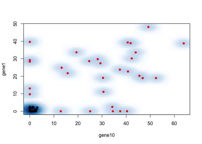
So for FACs, we would choose high gene1 or gene10 to sort for cells in group1!
Comparison
Let’s see how our results would be different if we just picked 2 most differentially expressed genes by a simple Wilcox rank sum test.
ct <- "group1"
## run wilcox test on all genes, get p value
wilcox.pv <- unlist(lapply(seq_along(rownames(mat)), function(g) {
    x <- mat[g, group[colnames(mat)]==ct]
    y <- mat[g, group[colnames(mat)]!=ct]
    pv <- wilcox.test(x, y, alternate="less")
    pv$p.val
}))
names(wilcox.pv) <- rownames(mat)
markers <- sort(wilcox.pv, decreasing=FALSE)
print(head(markers))
##       gene53       gene41       gene98       gene39        gene3
## 6.698431e-16 1.172235e-14 7.295158e-14 2.024959e-13 3.332489e-13
##       gene91
## 4.310527e-13
## take best 2 by p value
marker <- names(markers)[1:2]

## plot
smoothScatter(mat[marker[1],], mat[marker[2],],
              col=as.numeric(group[colnames(mat)]==ct)+1, pch=16,
              xlab=marker[1], ylab=marker[2])
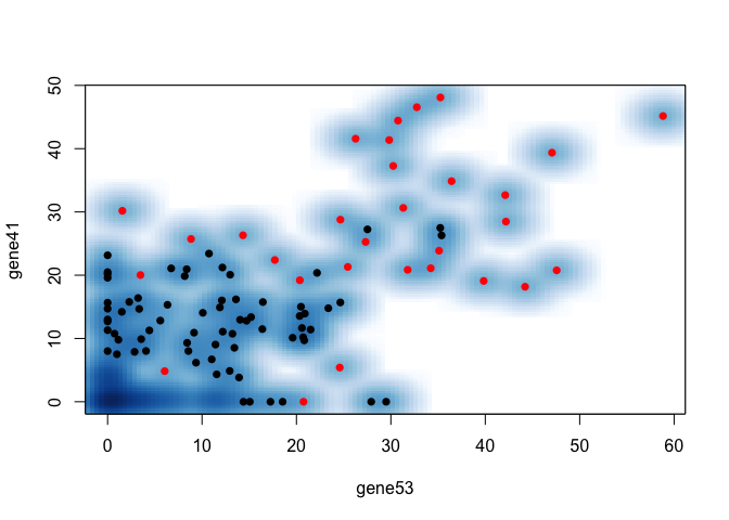
So it looks like our machine learning approach is better in this simulation. But of course, this is just a simulation. And in real life, we may have practical considerations like translation rate (not all highly expressed genes become highly expressed proteins) so there are likely other important information we currently don’t integrate in this approach. But consider: how do biologists pick which marker genes to use? Can we formulate that into some kind of machine learning approach? And how can we use machine learning to augment and inform what biologists are already doing?
Recent Posts
- AI-guided data visualization of gas prices in different geographical locations across the US over time on 04 May 2026
- The Mentorship Index on 01 March 2026
- Vibe coding with SEraster and STcompare to compare spatial transcriptomics technologies on 22 February 2026
- RNA velocity in situ infers gene expression dynamics using spatial transcriptomics data on 13 October 2025
- Analyzing ICE Arrest Data - Part 2 on 27 September 2025