Single-Cell RNA-seq Dimensionality Reduction with Deep Learning in R using Keras

Overview

In this tutorial, I walk through how to use the Keras package in R to do dimensionality reduction via autoencoders, focusing on single-cell RNA-seq data. I compare these results with dimensionality reduction achieved by more conventional approaches such as principal components analysis (PCA) and comment on the pros and cons of each.

Introduction

Single-cell RNA-seq data is highly dimensional; we are often looking at 1000s of genes and 100s to now millions of cells. In order to make sense of this high dimensional data, it often helps to project the data into a dimension we can visualize such as 2D or 3D. In such a 2D or 3D setting, as cells that are transcriptionally more similar to each other should be closer together, we should be able to better visualize transcriptionally distinct cell-types as distinguihable clusters. A number of single-cell RNA-seq dimensionality reduction and clustering approaches have been developed.

The problem

A hallmark of many of these current single-cell RNA-seq dimensionality reduction and clustering approaches is the reliance on variance. Specifically, methods will often first variance-normalize, select for genes that are more variable than expected, and apply prinicipal components analysis to extract the components of greatest variance, prior to finally embedding the data into a 2D or 3D visualization.

These steps are intended to improve signal and minimize noise. Indeed, for two large transcriptionally distinct cell-types, the genes that capture the most variance and likewise the prinicipal components that seek to maximize variance will best separate these two groups.

Consider the following simulation (adapted from our previous in-depth look on differential expression analysis)

# Simulate differentially expressed genes
set.seed(0)
G <- 3
N <- 30
M <- 1000
initmean <- 5
initvar <- 5
mat <- matrix(rnorm(N*M*G, initmean, initvar), M, N*G)
rownames(mat) <- paste0('gene', 1:M)
colnames(mat) <- paste0('cell', 1:(N*G))
group <- factor(sapply(1:G, function(x) { 
  rep(paste0('group', x), N)
}))
names(group) <- colnames(mat)
set.seed(0)
upreg <- 10
upregvar <- 5
ng <- 100
diff <- lapply(1:G, function(x) {
  diff <- rownames(mat)[(((x-1)*ng)+1):(((x-1)*ng)+ng)]
  mat[diff, group==paste0('group', x)] <<- 
    mat[diff, group==paste0('group', x)] + 
    rnorm(ng, upreg, upregvar)
  return(diff)
})
names(diff) <- paste0('group', 1:G)

## Positive expression only
mat[mat < 0] <- 0

## Visualize heatmap where each row is a gene, each column is a cell
## Column side color notes the cell-type
heatmap(mat, 
        Rowv=NA, Colv=NA, 
        col=colorRampPalette(c('blue', 'white', 'red'))(100), 
        scale="none", 
        ColSideColors=rainbow(G)[group], 
        labCol=FALSE, labRow=FALSE)

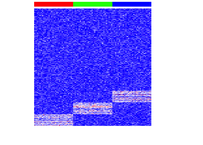
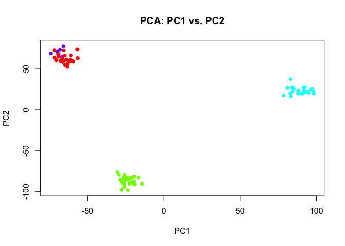
In this very simple simulation, we have 3 equally sized, transcriptionally distinct cell-types, each marked by the same number of uniquely upregulated genes. Now, we can see if PCA is able to project this high dimensional data into a lower number of dimensions for visualization.

pcs <- prcomp(t(mat))
plot(pcs$x[,1:2], 
     col=rainbow(G)[group], 
     pch=16, 
     main='PCA: PC1 vs. PC2')

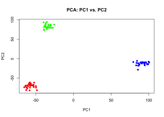
Indeed, PCA captures components of greatest variance that accurately separates the three populations of cells.

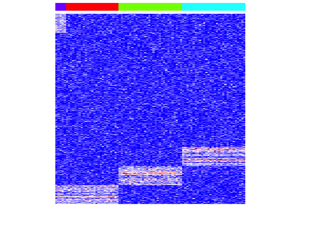
Now, let’s make things a little harder. Let’s add a population of 5 cells that are transcriptionally distinct but rare.

mat2 <- mat
mat2[(M-ng):M,1:5] <- mat[(M-ng):M,1:5]+upreg
diff$group4 <- rownames(mat2)[(M-ng):M]

group2 <- as.character(group)
group2[1:5] <- 'groupX'
names(group2) <- names(group)
group2 <- factor(group2)

heatmap(mat2, 
        Rowv=NA, Colv=NA, 
        col=colorRampPalette(c('blue', 'white', 'red'))(100), 
        scale="none", 
        ColSideColors=rainbow(length(levels(group2)))[group2], 
        labCol=FALSE, labRow=FALSE)

Keep in mind that PCA seeks to maximize global variance. Let’s look at the distirbution of variances for each set of differentially upregulated genes for each group. Group 4 is our rare cell-type.

genevar <- apply(mat2, 1, var)
par(mfrow=c(2,2))
hist(genevar[diff$group1], breaks=20, xlim=c(0,150))
hist(genevar[diff$group2], breaks=20, xlim=c(0,150))
hist(genevar[diff$group3], breaks=20, xlim=c(0,150))
hist(genevar[diff$group4], breaks=5, xlim=c(0,150))

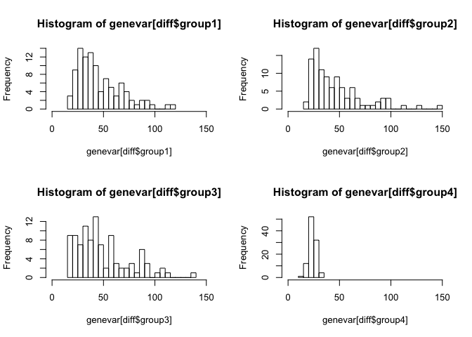
As expected, the genes driving the rare population are not as globally variable. As a result, the rare population is not apparent in the resulting dimensionality reduction visualization from the first 2 PCs.

pcs2 <- prcomp(t(mat2))
plot(pcs2$x[,c(1,2)], 
     col=rainbow(length(levels(group2)))[group2], 
     pch=16,
     main='PCA: PC1 vs. PC2')

Deep Learning

Now, let’s use deep learning instead. Specifically, we will use an autoencoder, a type of artificial neural network that we can use to learn a 2D representation (encoding) for our high dimensional single cell expression data. Specifically, the autoencoder will try to generate from the 2D reduced encoding a representation as close as possible to its original input. We can take advantage of this property to reason that the encoding layer must contain all the essential features (beyond just highly variable genes) that is important.

We will use the Keras package in R to train and test our autoencoder. For information on how to install Keras in R, see https://keras.rstudio.com/.

m <- as.matrix(t(mat2)) 
dim(m)

## [1]   90 1000

## scale from 0 to 1
range01 <- function(x){(x-min(x))/(max(x)-min(x))}
dat <- apply(m, 2, range01)
rownames(dat) <- rownames(m)
range(dat)

## [1] 0 1

dim(dat)

## [1]   90 1000

## train and test data are the same here
## ideally should split into separate train and test sets
## to avoid overfitting
x_train <- x_test <- dat

## Load Keras (https://keras.rstudio.com/)
library(keras)
K <- keras::backend()

## Deep learning model
input_size <- ncol(x_train) ## 1000 genes
hidden_size <- 10 ## 10 dimensional hidden layer
code_size <- 2 ## 2 dimensional encoding
input <- layer_input(shape=c(input_size))
hidden_1 <- layer_dense(input, hidden_size) %>% 
  layer_activation_leaky_relu() %>%
  layer_dropout(rate=0.1)
code <- layer_dense(hidden_1, code_size) %>% 
  layer_activation_leaky_relu()
hidden_2 <- layer_dense(code, units=hidden_size) %>% 
  layer_activation_leaky_relu()
output <- layer_dense(hidden_2, units=input_size, activation="sigmoid")

## input and output should be the same
autoencoder <- keras_model(input, output)
## encoder from input to code space
encoder <- keras_model(input, code)

## Learn
autoencoder  %>% compile(optimizer='adam', 
                         loss='cosine_proximity',
                         metrics='mae')
autoencoder %>% fit(
  x_train, x_train, 
  shuffle=TRUE, 
  epochs=1000, 
  batch_size=100, 
  validation_data=list(x_test, x_test)
)

############### Plot

## predict code space using deep learning  model
x_test_encoded <- predict(encoder, 
                          x_test, 
                          batch_size=100)
emb2 <- x_test_encoded
rownames(emb2) <- rownames(x_test)
colnames(emb2) <- c('latent 1', 'latent 2')

## plot
plot(emb2, 
     col=rainbow(length(levels(group2)))[group2], 
     pch=16,
     main='Autoencoder: 2D code layer')

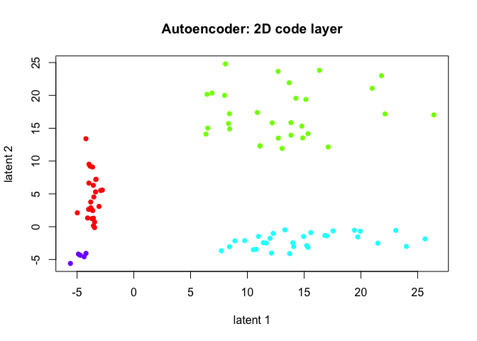
The autoencoder, given a sufficient number of epochs, does tease out the rare subpopulation.

Discussion

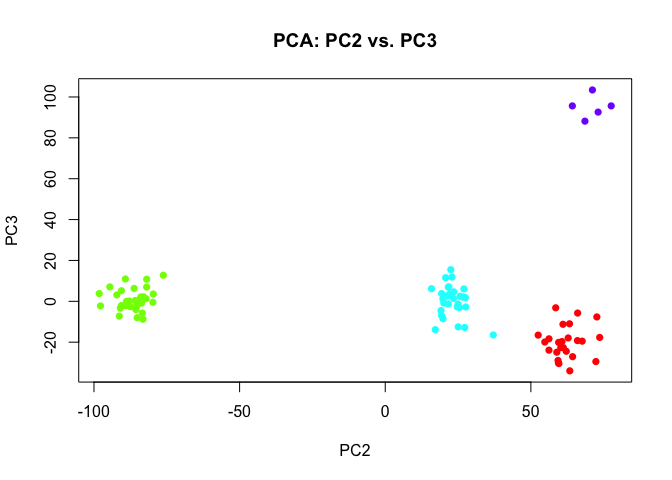
So are autoencoders inherently better for this problem then? Actually, if we just looked at more PCs, we would probably eventually find one that separates the rare subpopulation as well.

plot(pcs2$x[,c(2,3)], 
     col=rainbow(length(levels(group2)))[group2], 
     pch=16,
     main='PCA: PC2 vs. PC3')

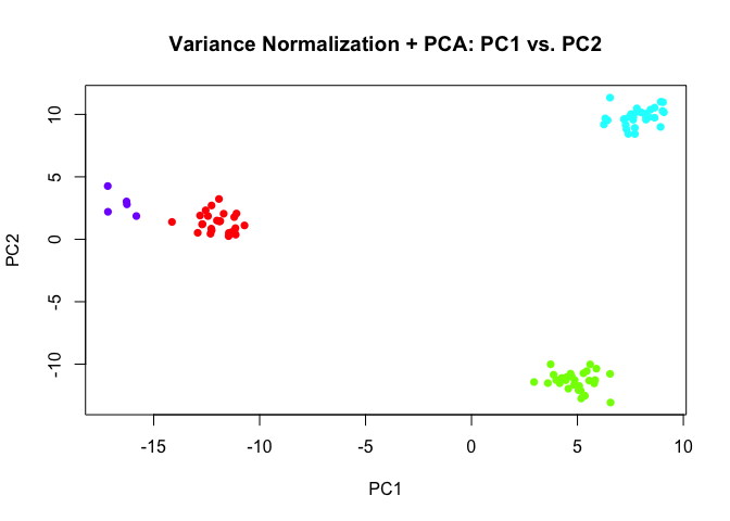
And likewise, had we introduced some variance normalization prior to PCA, we would have been able to tease out the rare subpopulations even in the first 2 PCs.

library(MUDAN)
## use all genes, not just significantly overdispersed
mat2norm <- normalizeVariance(mat2, alpha=1) 

## Converting to sparse matrix ...

## [1] "Calculating variance fit ..."
## [1] "Using gam with k=5..."
## [1] "1000 overdispersed genes ... "

pcs3 <- prcomp(t(mat2norm))
plot(pcs3$x[,1:2], 
     col=rainbow(length(levels(group2)))[group2], 
     pch=16,
     main='Variance Normalization + PCA: PC1 vs. PC2')

However, in real life, it is often not clear how many PCs we should look at. Additional technical artifacts may actually contribute more variance than genes driving a rare subpopulation. So a deep-learning-based approach in theory could provide a more unbiased (rather than being biased by variance) way to look for an underlying, representative 2D manifold that represents our data. But an unbiased approach may also pick on more technical variation that’s not biological interesting.

Still, the code or latent spaces derived by autoencoders are very difficult to interpret. A number of approaches have been developed to interactively explore and interpret these spaces; I really enjoyed tinkers with TL-GAN (transparent latent-space GAN) by Shaobo Guan. In contrast, for PCA, the loading values gives us interpretable information on the genes that contribute to each PC and are thus relevant for separating the cell-types.

Designing autoencoders is also an art in itself. Here, I only used one hidden layer, but I could have used as many as I wanted. I also used a particular loss function, activation function, and introduced dropout in each layer. These are all design choices that will dramatically impact your encoding and results!

So try it out for yourself!

• What happens if you include more hidden layers?
• What if you use a different loss function? Or different activation function?
• Does this work on real single-cell RNA-seq as opposed to simulated data?
• Alternatively, what if we use other non-variance based dimensionality reduction approaches like non-negative matrix factorization (NMF)? How does it compare?
• What if we use autoencoders to do dimensionality reduction into a 30 dimensional space instead of just 2D prior to using something like tSNE or UMAP to visualize a 2D space?