Complementing single-cell clustering analysis with MERINGUE spatial analysis

Jun 21, 2021

Introduction

We recently published a paper in the journal Genome Research on a new bioinformatics tool MERINGUE for characterizing spatial gene expression heterogeneity in spatially resolved single-cell transcriptomics data with nonuniform cellular densities. For more details about MERINGUE, please check out the paper or the code repository with tutorials on Github. In this blog post, I apply MERINGUE to new MERFISH data of the mouse cortex from Vizgen.

library(MERINGUE)

Background

The mamalian brain is made up of functionally distinct regions, comprising many transcriptionally distinct cell-types. The Allen Brain Atlas provides a cool tool for browsing these brain regions in mouse.

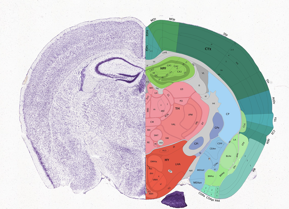
Characterizing how these transcriptionally distinct cell-types are spatially organized can help us understand how this spatial organization relates to function. This spatially resolved transcriptomics data with MERFISH profiles the expression of 483 genes in 3 full coronal slices of the mouse brain across 3 biological replicates.

Get the data

Here, we will focus on slice #2 replicate #1.

## read in data
cd <- read.csv('datasets_mouse_brain_map_BrainReceptorShowcase_Slice2_Replicate1_cell_by_gene_S2R1.csv.gz', row.names = 1)
annot <- read.csv('datasets_mouse_brain_map_BrainReceptorShowcase_Slice2_Replicate1_cell_metadata_S2R1.csv.gz', row.names = 1)
pos <- annot[, c('center_x', 'center_y')]
pos[,2] <- -pos[,2] ## flip Y coordinates

## visualize
par(mfrow=c(1,1))
MERINGUE::plotEmbedding(pos, unclassified.cell.color='black', cex=0.1)

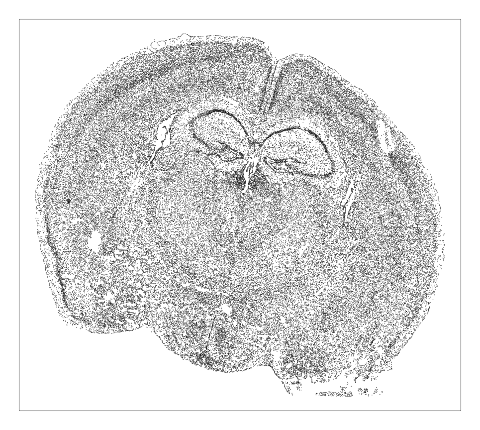
Each point is a cell. So based on density alone, we can already see some interesting spatial organization. Let’s use clustering analysis to identify transcriptionally distinct cell-types.

Single-cell Clustering Analysis

We are interested in identifying genes that exhibit significant spatial heterogeneity. However, given that transcriptionally distinct cell-types are spatially organized in the brain, a lot of the significant spatial heterogeneity we identify will be driven by this underlying spatial organization of cell-types. So let’s first identify cell-types and see how they’re spatially organized and then look for additional aspects of spatial heterogeneity within cell-types.

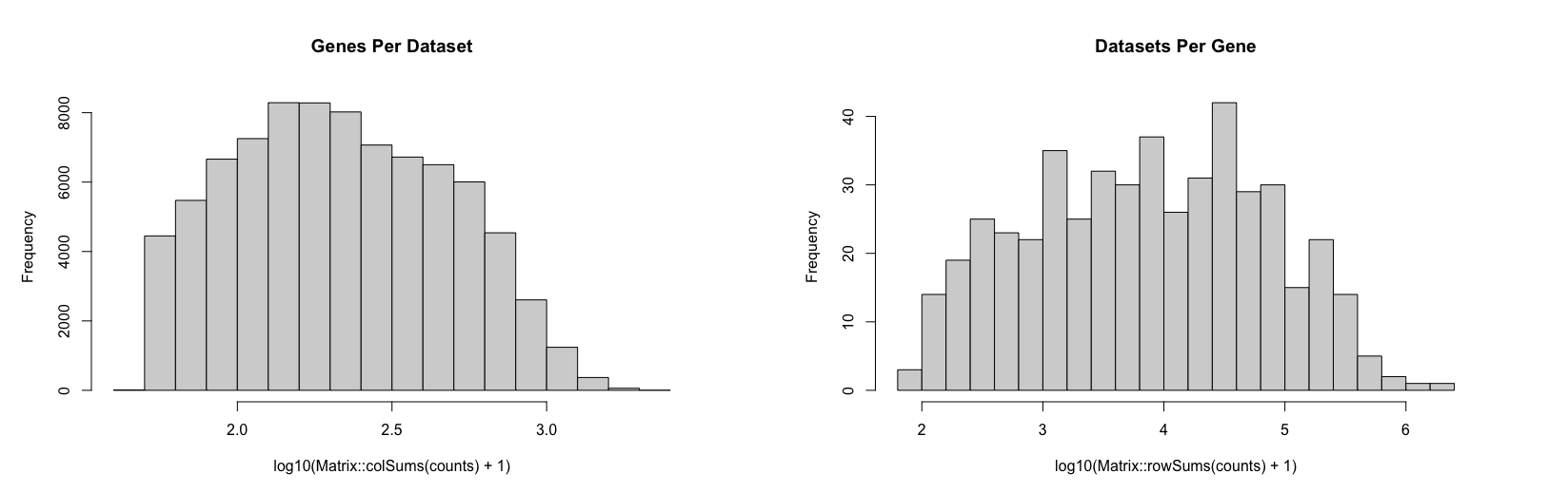
First, let’s remove blank control barcodes from the MERFISH dataset as well as poor genes and cells with few reads as needed.

## remove blanks
good.genes <- colnames(cd)[!grepl('Blank', colnames(cd))]
counts <- t(cd[, good.genes])
## filter
counts <- MERINGUE::cleanCounts(counts, verbose = FALSE)

There are many ways to identify cell-types via different types of single-cell clustering analysis. Here, we will just do a quick and dirty CPM normalization, followed by PCA dimensionality reduction, and graph based clustering. We can visualize the results using UMAP as well as on our original spatial coordinates.

## CPM normalize, log transform
mat <- MERINGUE::normalizeCounts(counts, log = TRUE)
dim(mat)
## pca, take top 30 PCs
## note to self: slow, need to find faster pca
#pcs <- irlba::prcomp_irlba(mat, n=30) 
## update: RSpectra svds is much faster so switch to that
pca <- RSpectra::svds(A = t(mat), k=30,
                      opts = list(center = TRUE, scale = FALSE, maxitr = 2000, tol = 1e-10))
foo <- as.matrix(t(mat) %*% pca$v[,1:30])
rownames(foo) <- colnames(mat)
## graphic based clustering on PC loadings
## subsample down to 10% of cells and infer rest to speed up
com <- MUDAN::getApproxComMembership(foo, k=10,
                                     nsubsample = nrow(foo)*0.1,
                                     method=igraph::cluster_louvain)
table(com)

## UMAP
emb <- uwot::umap(foo)
rownames(emb) <- colnames(mat)
dim(emb)

## plot
par(mfrow=c(1,1))
MERINGUE::plotEmbedding(emb, groups=com,
                        show.legend=TRUE, legend.x = "topleft",
                        mark.clusters = TRUE,
                        cex=0.1, main='UMAP')
MERINGUE::plotEmbedding(pos, groups=com,
                        cex=0.2, main='Spatial')

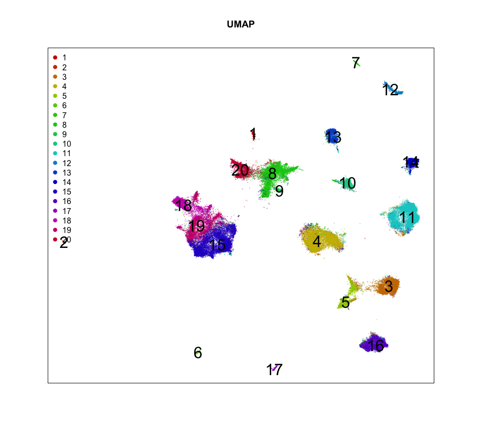
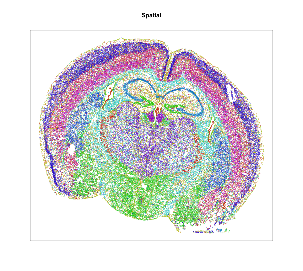
So it looks like we can identify 20 transcriptionally distinct clusters or cell-types here. And they have seem to have pretty distinct spatial organizations. Neat!

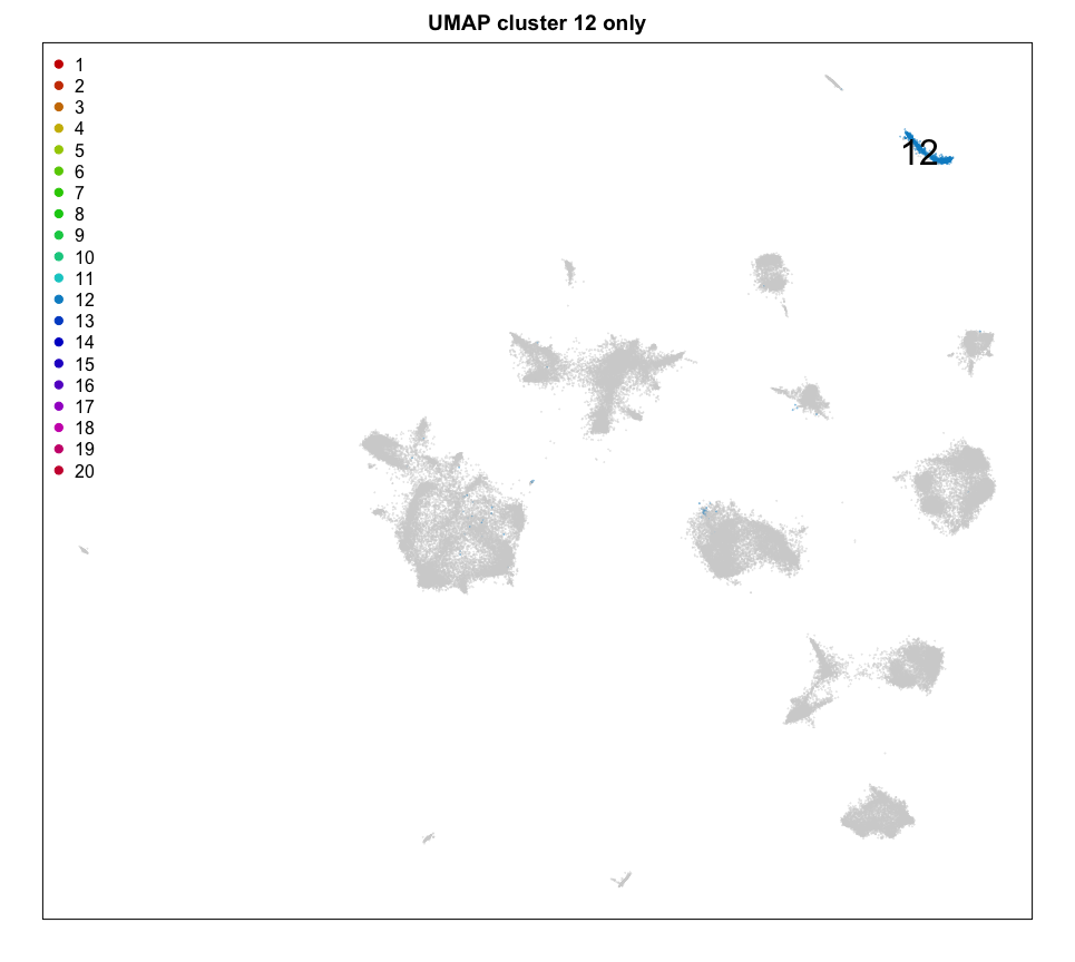
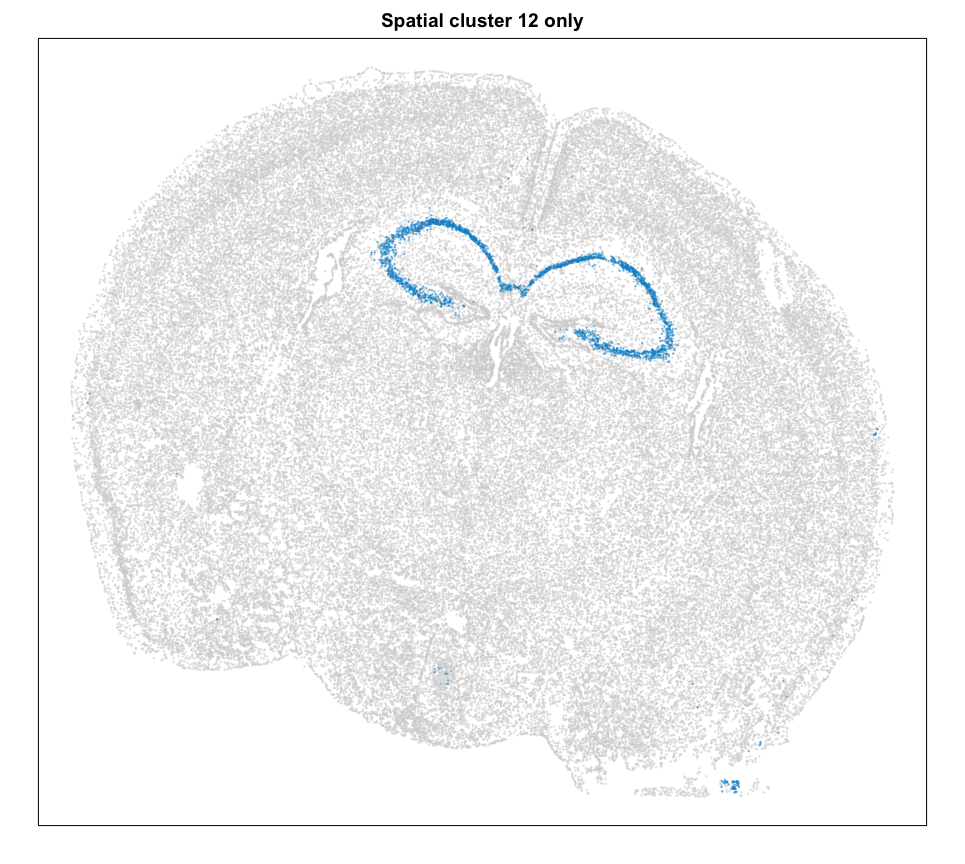
Let’s focus on the cells of cluster 12 for now. Based on its spatial organization, perhaps this cluster corresponds to pyramidal neurons.

ct = 12 ## pyrimidal layer
cells <- names(com)[com == ct]

par(mfrow=c(1,1))
MERINGUE::plotEmbedding(emb, groups=com[cells],
                        show.legend = TRUE, legend.x = "topleft",
                        mark.clusters = TRUE,
                        cex = 0.1, main = 'UMAP cluster 12 only')
MERINGUE::plotEmbedding(pos, groups=com[cells],
                        cex = 0.2, main = 'Spatial cluster 12 only')
			
posh <- pos[cells,]
dim(posh)
math <- mat[, cells]

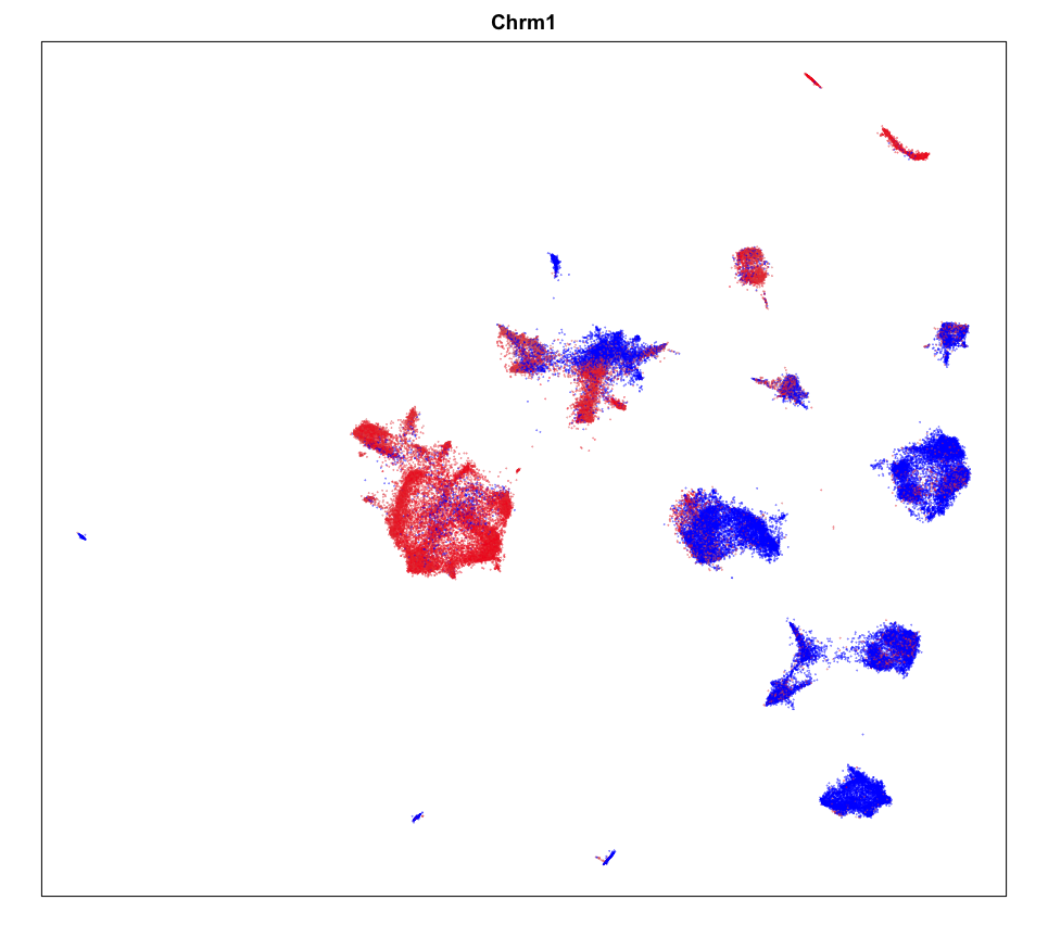
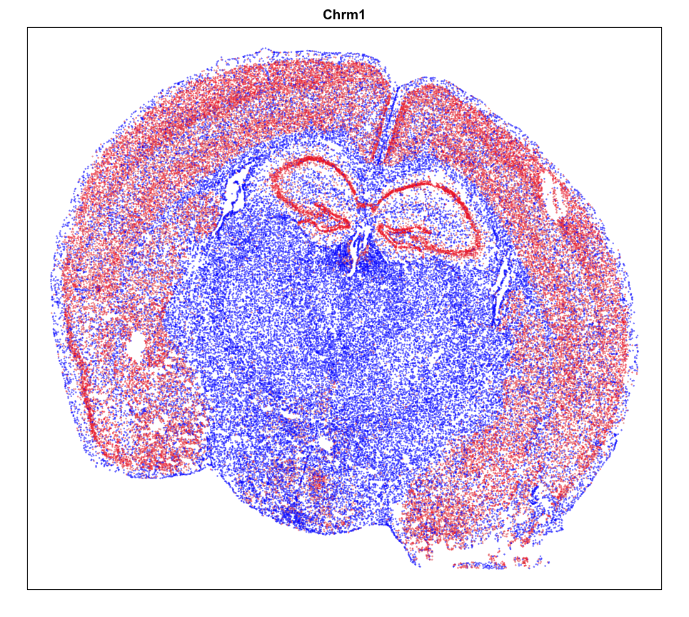
We can plot a few marker genes to confirm as well.

dg <- MERINGUE::getDifferentialGenes(mat, com)
head(dg[[12]][order(dg[[12]]$Z, decreasing=TRUE),], n=20)

## manually pick a few
## https://www.proteinatlas.org/ENSG00000168539-CHRM1
g <- 'Chrm1'
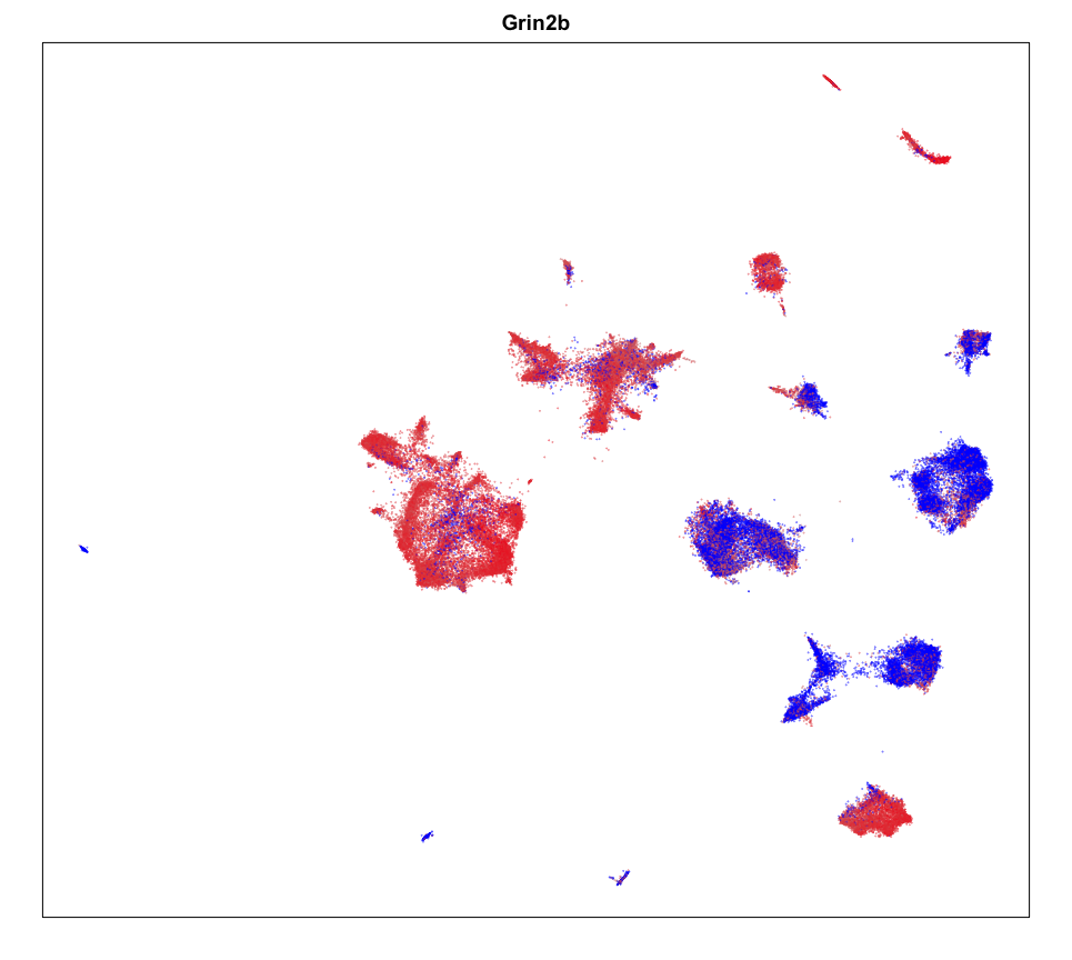
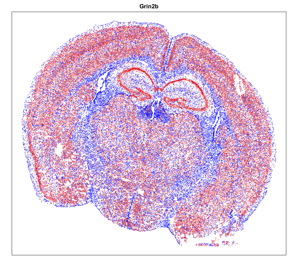
## https://www.proteinatlas.org/ENSG00000273079-GRIN2B
g <- 'Grin2b'
gexp <- mat[g,]
gexp <- scale(gexp)[,1]
gexp[gexp > 1.5] <- 1.5
gexp[gexp < -1.5] <- -1.5
par(mfrow=c(1,1))
MERINGUE::plotEmbedding(emb, col=gexp,
                        cex = 0.1, main = g)
MERINGUE::plotEmbedding(pos, col=gexp,
                        cex = 0.2, main = g)

Spatial Analysis

Focusing on cluster 12 cells, we can use MERINGUE to identify significantly spatially variable genes driven by more than 10% of cells.

## Get neighbor-relationships
#W <- MERINGUE::getSpatialNeighbors(posh[1:50,], filterDist = 50)
#MERINGUE::plotNetwork(posh[1:50,], W)
W <- MERINGUE::getSpatialNeighbors(posh, filterDist = 50)

## Get spatial patterns
I <- MERINGUE::getSpatialPatterns(math, W)
## Filter for patterns driven by > 10% of cells
results.filter <- MERINGUE::filterSpatialPatterns(mat = math,
                                                  I = I,
                                                  w = W,
                                                  adjustPv = TRUE,
                                                  alpha = 0.05,
                                                  minPercentCells = 0.10,
                                                  verbose = FALSE,
                                                  details=TRUE)

We identify 39 such genes. We can further see how these genes comprise spatially distinct patterns.

# Identify primary patterns
scc <- MERINGUE::spatialCrossCorMatrix(mat = as.matrix(math[rownames(results.filter),]),
                                       weight = W)
par(mfrow=c(1,3), mar=rep(2,4))
ggroup <- MERINGUE::groupSigSpatialPatterns(pos = pos,
                                            mat = as.matrix(math[rownames(results.filter),]),
                                            scc = scc,
                                            power = 1,
                                            hclustMethod = 'ward.D',
                                            deepSplit = 1,
                                            zlim=c(-1.5,1.5))
                                            

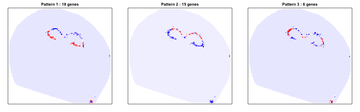
We can also look at specific genes within each pattern to appreciate their spatial expression distribution.

par(mfrow=c(3,3), mar=rep(2,4))
# Look at specific genes in each groups
lapply(levels(ggroup$groups), function(gr) {
  gs <- names(ggroup$groups)[ggroup$groups == gr]
  ## select few driven by most cells
  gs <- gs[order(results.filter[gs,]$minPercentCells, decreasing=TRUE)][1:3]
  lapply(gs, function(g) {
    ## z-score expression within cluster 12 cells
    gexp <- math[g,]
    gexp <- scale(gexp)[,1]
    gexp[gexp > 1.5] <- 1.5
    gexp[gexp < -1.5] <- -1.5
    ## set as NAs for rest
    gexpall <- rep(NA, nrow(pos))
    names(gexpall) <- rownames(pos)
    gexpall[names(gexp)] <- gexp
    MERINGUE::plotEmbedding(pos, col=gexpall, main=g, cex=0.05)
  })
})

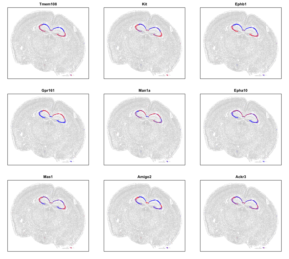
Visually, these patterns appear to match the organization of the CA3, CA2, CA1 regions, which we know to be comprised of pyrimidal cells that differ in theirs of their neural inputs and outputs. Cool!

Try it out for yourself!

Try out the analysis for a different cell-type.
Are identified spatial patterns bilaterally symmetric? Can we quantify this?
Do certain genes exhibit spatial heterogeneity in multiple cell-types? What are these genes? Are they enriched for certain functional classifications? Are their spatial patterns consistents across cell-types?

SEARCH

EXPLORE MORE POSTS

by Tags | by Date