Aligning 10X Visium spatial transcriptomics datasets using STalign with Reticulate in R

In this blog post, I will use our recently developed tool STalign to align two 10X Visium spatial transcriptomics datasets from Dixon et al (JASN, 2022). While STalign is implemented in Python, I prefer working in R so I will use the reticulate R package to interface with Python from within RStudio with Rmarkdown.

Introduction

Spatial transcriptomics (ST) technologies enable us to measure spatially-resolved gene expression within thin tissue slices. When we apply ST to profile tissues across different diseased settings, we may be interested in evaluating gene expression differences at spatial locations across structurally matching tissue regions. Such spatial comparisons demand alignment of these ST datasets.

As we’ve explored in previous blog posts, we can use STalign to align ST data of structurally similar tissues from different single-cell resolution spatial transcriptomics technologies. Using simulations, we can highlight how STalign is able to achieve highly accurate alignments, accommodating non-linear structural variation that may be due to biological heterogeneity and/or induced during the experimental data collection process.

As further detailed in our bioRxiv preprint, STalign is also able ST datasets from multi-cellular pixel-resolution ST technologies such as 10X Visium using the corresponding registered single-cell resolution histology image. The transformation learned from aligning the histology images can be applied to move the Visium spots into the aligned coordinate space to enable downstream spatial comparative analysis.

Here, we will use STalign to align two 10X Visium datasets of the mouse kidney from different timepoints of renal ischemia-reperfusion injury from Dixon et al (JASN, 2022). Feel free to download the data from the (Re)Building a Kidney Consortium database and follow along for yourself.

Setting up

I am running everything in RStudio using Rmarkdown (screenshot below).

I have already installed matplotlib, numpy, and other dependencies for my base Python3 instance. Likewise, I have already installed reticulate within R. So I will create an Rmarkdown codeblock to use R to load reticulate and activate this base Python3 version and associated modules.

# R codeblock -----
library(reticulate)
use_condaenv("base")

I have already cloned the STalign Github repo to my Desktop. So I will create an Rmarkdown codeblock to use Python to just source the STalign.py script.

# Python codeblock -----
import sys
sys.path.append("~/Desktop/STalign/STalign/")
import STalign

For this tutorial, we will align two 10X Visium datasets of coronal sections of mouse kidney. These kidney sections have enough structural similarity to enable such alignment. I will focus on the datasets corresponding to the 12-hour and 2-day injury timepoints. I generally prefer reading, writing, and processing matrices in R so I will read the relevant spatial data into R.

# R codeblock -----
library("rjson")

AKI_12h_pos <- read.csv('Female_AKI_12hAKI_3_1_processed/outs/spatial/tissue_positions_list.csv', header = FALSE, row.names=1)
AKI_12h_barcodes <- read.csv('Female_AKI_12hAKI_3_1_processed/outs/filtered_feature_bc_matrix/barcodes.tsv.gz')
AKI_12h_scalefactor <- fromJSON(file='Female_AKI_12hAKI_3_1_processed/outs/spatial/scalefactors_json.json')$tissue_hires_scalef

AKI_2d_pos <- read.csv('Female_AKI_2dayAKI_4_1_processed/outs/spatial/tissue_positions_list.csv', header = FALSE, row.names=1)
AKI_2d_barcodes <- read.csv('Female_AKI_2dayAKI_4_1_processed/outs/filtered_feature_bc_matrix/barcodes.tsv.gz')
AKI_2d_scalefactor <- fromJSON(file='Female_AKI_2dayAKI_4_1_processed/outs/spatial/scalefactors_json.json')$tissue_hires_scalef

Visualizing the data before alignment

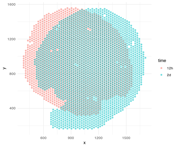
Now we can plot the positions of the Visium spots. I prefer plotting within R using packages like ggplot2. I will filter for spots that are on the tissue based on the barcodes included in the filtered_feature_bc_matrix matrix. I will also use the scalefactors in scalefactors_json.json to scale the spot positions into more interpretable units that are consistent with the histology image later.

# R codeblock -----
library(ggplot2)

pos1 <- AKI_12h_pos[AKI_12h_barcodes[,1],5:4] * AKI_12h_scalefactor
pos2 <- AKI_2d_pos[AKI_2d_barcodes[,1],5:4] * AKI_2d_scalefactor
colnames(pos1) <- colnames(pos2) <- c('x', 'y')

df <- data.frame(rbind(cbind(pos1, time='12h'), cbind(pos2, time='2d')))
ggplot(df, aes(x=x, y=y, col=time)) + geom_point(alpha=0.5) + theme_minimal()

Both sets of pixel-resolution Visium spots are registered to a corresponding single-cell resolution histology image. We will use STalign to solve for a transformation that when applied to the one histology image (we will call the “source”) will make it look like the other histology image (we will call the “target”). Once we learn this transformation, we can apply them to the spots to move the spots into the aligned coordinate system. Please check out our bioRxiv preprint for more details on how this is done.

STalign is implemented in Python. So I will read the histology images into Python and use STalign to normalize their image intensities for downstream purposes.

# Python codeblock -----
import matplotlib.pyplot as plt

## source
image_file = 'Female_AKI_12hAKI_3_1_processed/outs/spatial/tissue_hires_image.png'
V = plt.imread(image_file)
Inorm = STalign.normalize(V)

## target
image_file = 'Female_AKI_2dayAKI_4_1_processed/outs/spatial/tissue_hires_image.png'
G = plt.imread(image_file)
Jnorm = STalign.normalize(G)

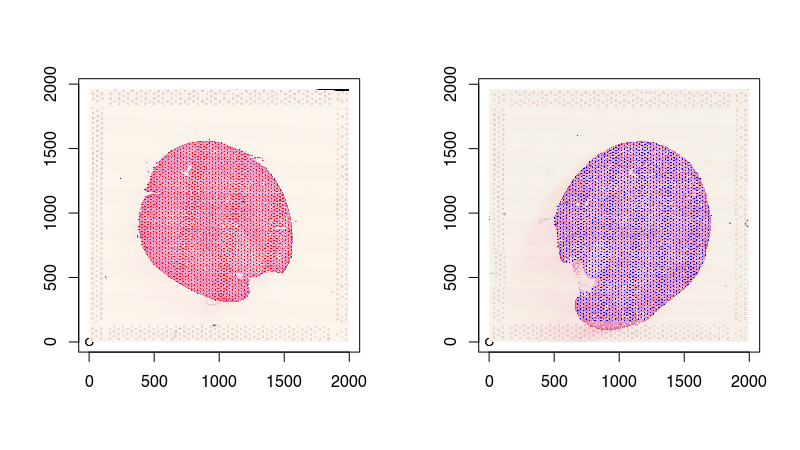
Eventhough I’ve read the images into Python so they can be normalized by STalign, I still prefer to plotting in R. Because we are using reticulate, we can access these images in R! And since we read our Visium spot positions into R previously, now we can plot both on top of each other to confirm that the Visium spots have been registered to their corresponding single-cell resolution histology images.

# R codeblock -----
par(mfrow=c(1,2))

## source
plot(c(0,0), xlim=c(0,ncol(py$Inorm)), ylim=c(0,nrow(py$Inorm)),
	    xlab=NA, ylab=NA)
rasterImage(py$Inorm, xleft = 0, xright = ncol(py$Inorm),
            ytop = 0, ybottom = nrow(py$Inorm), interpolate = FALSE)
	    points(pos1, pch=16, cex=0.2, col='red')

## target
plot(c(0,0), xlim=c(0,ncol(py$Jnorm)), ylim=c(0,nrow(py$Jnorm)),
	    xlab=NA, ylab=NA)
rasterImage(py$Jnorm, xleft = 0, xright = ncol(py$Jnorm),
            ytop = 0, ybottom = nrow(py$Jnorm), interpolate = FALSE)
	    points(pos2, pch=16, cex=0.2, col='blue')

Aligning with STalign

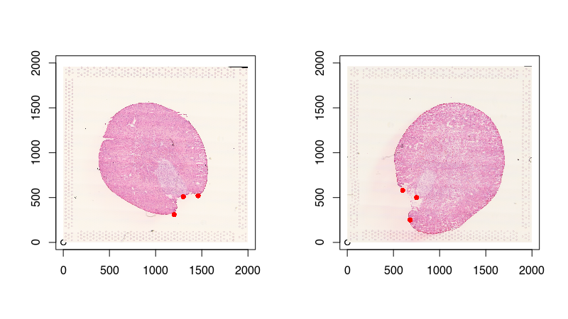
To assist with the spatial alignment, I will place a few landmark points. This will help mitigate the likelihood of us falling into a local minimum in the gradient descent and arrive at a suboptimal solution. I will just manually create them by eyeballing the image. They can be very approximate as STalign will integrate these landmarks with other imaging features in its optimization. Again, please check out the online supplementary methods bioRxiv preprint for more details.

# R codeblock -----
par(mfrow=c(1, 2))

## source
pointsI <- t(data.frame(a = c(1300, 510), b = c(1460, 520), c = c(1200, 310))); colnames(pointsI) <- c('x', 'y')
plot(c(0,0), xlim=c(0,2000), ylim=c(0,2000),  xlab=NA, ylab=NA)
rasterImage(py$Inorm, xleft = 0, xright = ncol(py$Inorm),
            ytop = 0, ybottom = nrow(py$Inorm), interpolate = FALSE)
	    points(pointsI, col='red', pch=16)

## target
pointsJ <- t(data.frame(a = c(750, 500), b = c(680, 250), c = c(600, 580))); colnames(pointsI) <- c('x', 'y')
plot(c(0,0), xlim=c(0,2000), ylim=c(0,2000),  xlab=NA, ylab=NA)
rasterImage(py$Jnorm, xleft = 0, xright = ncol(py$Jnorm),
            ytop = 0, ybottom = nrow(py$Jnorm), interpolate = FALSE)
	    points(pointsJ, col='red', pch=16)

The trickiest part of switching back and forth between R and Python in my opinion is keeping track of the coordinates! STalign with tensors in Python use row-column designation while position coordinates in R use x-y. I am personally much more comfortable with matrix operations like subsetting and swapping orders in R, so let’s just do these things in R to make our lives in Python easier later.

# R codeblock -----

# switch to row col order
pointsIrc = pointsI[,2:1]
pointsJrc = pointsJ[,2:1]

# split so we can access them more easily in Python later
xI <- pos1[,1]
yI <- pos1[,2]
xJ <- pos2[,1]
yJ <- pos2[,2]

Now let’s run the actual alignment with STalign. There are many Python Jupyter notebooks you can reference to copy over the relevant Python codeblocks. Note how we can access the landmark points pointsIrc and pointsJrc we created in R now in Python using reticulate! We will use these landmarks to compute an initial affine transformation.

# Python codeblock -----

# compute initial affine transformation from points
L,T = STalign.L_T_from_points(r.pointsIrc, r.pointsJrc)

# transpose matrices into right dimensions, set up extent
I = Inorm.transpose(2,0,1)
YI = np.array(range(I.shape[1]))*1. # needs to be longs not doubles for STalign.transform later so multiply by 1.
XI = np.array(range(I.shape[2]))*1. # needs to be longs not doubles for STalign.transform later so multiply by 1.
extentI = STalign.extent_from_x((YI,XI))

J = Jnorm.transpose(2,0,1)
YJ = np.array(range(J.shape[1]))*1. # needs to be longs not doubles for STalign.transform later so multiply by 1.
XJ = np.array(range(J.shape[2]))*1. # needs to be longs not doubles for STalign.transform later so multiply by 1.
extentJ = STalign.extent_from_x((YJ,XJ))

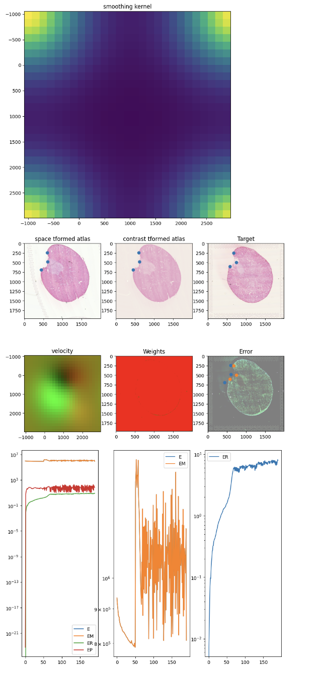
Now we can run STalign to align our “source image” I corresponding to the histology image from the 12h mouse kidney and our “target image” J corresponding to the histology image from the 2d mouse kidney. There are a few parameters that may need to be tuned depending on the size of your tissue and the degree of local diffeomorphism you want to tolerate (such as the smoothness scale of velocity field a), and how long you want to run the algorithm for (such as the number of iterations in the gradient descent niter and the step size epV). There are many Python Jupyter notebooks you can reference to see the range of different parameters that may be used.

# Python codeblock -----
torch.set_default_device('cpu')
device = 'cpu'

# keep all other parameters default
params = {'L':L,'T':T,
       'niter':100,
       'pointsI':r.pointsIrc,
       'pointsJ':r.pointsJrc,
       'device':device,
       'sigmaM':0.15,
       'sigmaB':0.2,
       'sigmaA':0.3,
       'a':300,
       'epV':10,
       'muB': torch.tensor([251,245,235]) # white is background
}

# run LDDMM
out = STalign.LDDMM([YI,XI],I,[YJ,XJ],J,**params)

# get necessary output variables
A = out['A']
v = out['v']
xv = out['xv']

After aligning, we can apply the learned transform, which includes both an affine and diffeomorphic component, to move the spatial positions of our Visium spots from the source dataset (the 12h mouse kidney) to be aligned with the target (the 2d mouse kidney).

# Python codeblock -----
tpointsI = STalign.transform_points_source_to_target(xv,v,A,np.stack([r.yI, r.xI], -1)) # transform the points
tpointsI = tpointsI.numpy() # convert from tensor to numpy to access in R later

Visualizing the results after alignment

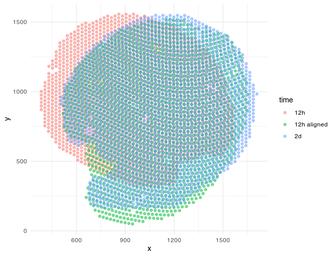
Now that we’re done aligning with STalign in Python, I can use reticulate to access these new aligned spot positions tpointsI in R and plot again using ggplot2!

# R codeblock -----
posAligned <- py$tpointsI ## currently in row-col order
posAligned <- data.frame(posAligned[,2:1]) ## put into x-y order
rownames(posAligned) <- rownames(pos1)
colnames(posAligned) <- c('x', 'y')

df <- data.frame(rbind(cbind(pos1, time='12h'),
      		       cbind(posAligned, time='12h aligned'),
   		       cbind(pos2, time='2d')))
ggplot(df, aes(x=x, y=y, col=time)) + geom_point(alpha=0.5) + theme_minimal()

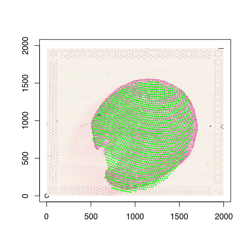
We can also visualize the new aligned Visium spot positions, which recall is from the 12h mouse kidney, onto the target histology image, which is from the the 2d mouse kidney. And indeed we see a pretty good spatial correspondence!

# R codeblock -----
par(mfrow=c(1,1))
plot(c(0,0), xlim=c(0,2000), ylim=c(0,2000),  xlab=NA, ylab=NA)
## target
rasterImage(py$Jnorm, xleft = 0, xright = ncol(py$Jnorm),
            ytop = 0, ybottom = nrow(py$Jnorm), interpolate = FALSE)

## aligned
points(posAligned, cex=0.4, col='green', pch=16)

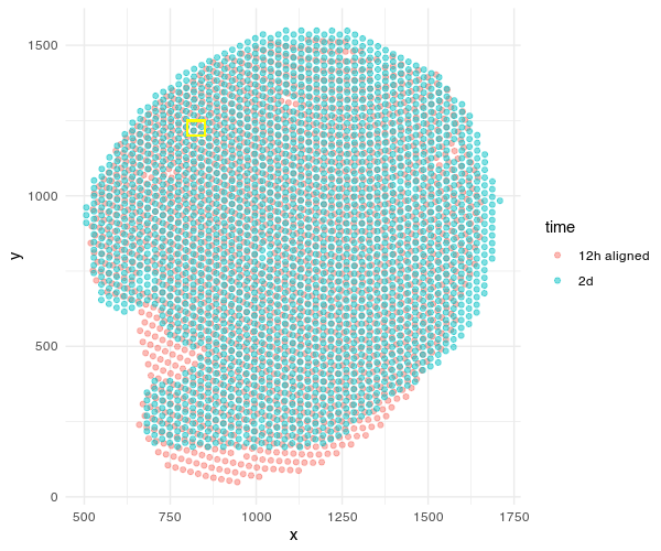
Given these aligned Visium spots, we can begin making gene expression and even cell-type compositional comparisons at spatially aligned spatial locations such as a particular region of the renal medulla, etc.

# R codeblock -----

# mark region of interest
df <- data.frame(rbind(cbind(posAligned, time='12h aligned'),
      		       cbind(pos2, time='2d')))
ggplot(df, aes(x=x, y=y, col=time)) +
	   geom_point(alpha=0.5) +
	   theme_minimal() +
  	   geom_rect(aes(xmin = 800, xmax = 850, ymin = 1200, ymax = 1250),
	   	       color = 'yellow', fill = NA, alpha=0.2)

# Try it out for yourself: see if you can grab the spots in this region and compare the gene expression profiles across 12h and 2d!

Perhaps making such comparisons will be the topic of a future blog post!

Try it out for yourself!

• This alignment can still be improved! In particular, the ureter/pelvis region may need some additional landmarks to guide alignment or parameter tuning to allow for finer local diffeomorphisms. See if you can achieve a better structural alignment!
• Try out different parameters for running STalign. What happens if you decrease a for example?
• How do the aligned Visium spot locations compare to if you performed a manual affine alignment by just translating the spots left/right/up/down, rotating, etc?
• What happens if you were to align the 2d mouse kidney to the 12h? ie. swap the order of the source and target.