Characterizing spatial heterogeneity using spatial bootstrapping with SEraster
SEraster aggregates single cell spatial omics data into square/hex pixels for scalable analysis
We recently developed an R package to perform rasterization
preprocessing for spatial omics data called
SEraster. The details of
the framework can be found in our Bioinformatics
paper.
Briefly, SEraster aggregates information in spatial omics data
into non-overlapping, spatial contiguous, square or hexagonal pixels to
speed up and enable other downstream analyses. In our paper, we
demonstrate how SEraster can be applied to effectively speed up
spatial variable gene expression analysis as well as enable the
characterization of cell-type co-enrichment. However, as we have seen
in other blog
posts,
if we can understand the principles underlying a computational method,
we can often apply it to achieve analyses not originally demonstrated.
In this blog post, I will show how I use SEraster to perform spatial
bootstrapping in order to characterize the variability of cell-type
proportions estimates as a function of tissue section size. In
particular, I am interested in characterizing the proportional
representation of cell-types in a tissue However, my cell-type
proportion estimates may be different depending on my tissue section.
But how variable are these estimates? This will depend on aspects of the
tissue such as the “representative-ness” of each section, which will
likely vary depending on the structures inherent in the tissue and the
size of our tissue section. So I will use spatial transcriptomics and
SEraster to evaluate.
Reading in spatial CosMx transcriptomics data
Let’s consider a CosMx SMI Human Liver FFPE spatial transcriptomics dataset from Nanostring (you can download the rather large Seurat object available through the Nanostring website and follow along yourself). Using the gene expression information associated with each cell, the cells have already been clustered and annotated with cell-type names.
Conveniently for me, we already processed this dataset as part of our other paper benchmarking different normalization methods for imaging-based spatial transcriptomics data, so I will simply load in the components I need, which is just the cell-type annotations and cell positions for one tissue section.
## read in data
meta <- readRDS('~/OneDrive - Johns Hopkins/CosMx_liver/data_from_website/cosmx_liver_meta.RDS')
## restrict to one sample of interest
vi <- meta$Run_Tissue_name == 'NormalLiver'
meta <- meta[vi,]
head(meta)
##              RNA_pca_cluster_default RNA_pca_cluster_default.1 orig.ident
## c_1_100_10                        13                        15          c
## c_1_100_1078                       7                        11          c
## c_1_100_1135                      12                        10          c
## c_1_100_267                       15                        17          c
## c_1_100_732                       12                        10          c
## c_1_100_909                       12                        19          c
##              nCount_RNA nFeature_RNA nCount_negprobes nFeature_negprobes
## c_1_100_10           33           26                0                  0
## c_1_100_1078       1699          295                0                  0
## c_1_100_1135        173          131                1                  1
## c_1_100_267         675          204                2                  2
## c_1_100_732         241          167                3                  3
## c_1_100_909         300          193                2                  2
##              nCount_falsecode nFeature_falsecode fov  Area AspectRatio Width
## c_1_100_10                  5                  5 100  2430        1.21    63
## c_1_100_1078                7                  7 100 17657        1.80   227
## c_1_100_1135                9                  8 100  9382        1.08   121
## c_1_100_267                 3                  3 100 15449        1.04   166
## c_1_100_732                16                 16 100 11206        1.41   145
## c_1_100_909                20                 18 100 10987        1.52   188
##              Height Mean.PanCK Max.PanCK Mean.CK8.18 Max.CK8.18 Mean.Membrane
## c_1_100_10       52        363      1121          23        274           259
## c_1_100_1078    126        355      1463        1512       6231           384
## c_1_100_1135    112        321      1319         246       3745           699
## c_1_100_267     159        222       907         800       6121           544
## c_1_100_732     103        786      2223         545       2486          1058
## c_1_100_909     124        615      1633         551       5889           903
##              Max.Membrane Mean.CD45 Max.CD45 Mean.DAPI Max.DAPI      cell_id
## c_1_100_10            911       137      504       457     1508   c_1_100_10
## c_1_100_1078         2110       143      845      3758    16112 c_1_100_1078
## c_1_100_1135         5260       319     3083      3459    14700 c_1_100_1135
## c_1_100_267          3993        61     4755      3710    21732  c_1_100_267
## c_1_100_732          3016       385     3384      4323    20568  c_1_100_732
## c_1_100_909          9566       518     6120      2815    17932  c_1_100_909
##              assay_type Run_name slide_ID_numeric Run_Tissue_name    Panel
## c_1_100_10          RNA        ?                1     NormalLiver 1000plex
## c_1_100_1078        RNA        ?                1     NormalLiver 1000plex
## c_1_100_1135        RNA        ?                1     NormalLiver 1000plex
## c_1_100_267         RNA        ?                1     NormalLiver 1000plex
## c_1_100_732         RNA        ?                1     NormalLiver 1000plex
## c_1_100_909         RNA        ?                1     NormalLiver 1000plex
##              Mean.Yellow Max.Yellow Mean.CD298_B2M Max.CD298_B2M      cell_ID
## c_1_100_10            NA         NA             NA            NA   c_1_100_10
## c_1_100_1078          NA         NA             NA            NA c_1_100_1078
## c_1_100_1135          NA         NA             NA            NA c_1_100_1135
## c_1_100_267           NA         NA             NA            NA  c_1_100_267
## c_1_100_732           NA         NA             NA            NA  c_1_100_732
## c_1_100_909           NA         NA             NA            NA  c_1_100_909
##              x_FOV_px y_FOV_px x_slide_mm y_slide_mm propNegative complexity
## c_1_100_10       2737       25    9.03144    9.73500  0.000000000   1.269231
## c_1_100_1078      595     3998    8.77440    9.25824  0.000000000   5.759322
## c_1_100_1135     1469     4199    8.87928    9.23412  0.005747126   1.320611
## c_1_100_267      3486     1058    9.12132    9.61104  0.002954210   3.308824
## c_1_100_732      3178     2771    9.08436    9.40548  0.012295082   1.443114
## c_1_100_909      3643     3429    9.14016    9.32652  0.006622517   1.554404
##              errorCtEstimate percOfDataFromError qcFlagsRNACounts
## c_1_100_10                 0           0.0000000             Pass
## c_1_100_1078               0           0.0000000             Pass
## c_1_100_1135             100           0.5780347             Pass
## c_1_100_267              200           0.2962963             Pass
## c_1_100_732              300           1.2448133             Pass
## c_1_100_909              200           0.6666667             Pass
##              qcFlagsCellCounts qcFlagsCellPropNeg qcFlagsCellComplex
## c_1_100_10                Pass               Pass               Pass
## c_1_100_1078              Pass               Pass               Pass
## c_1_100_1135              Pass               Pass               Pass
## c_1_100_267               Pass               Pass               Pass
## c_1_100_732               Pass               Pass               Pass
## c_1_100_909               Pass               Pass               Pass
##              qcFlagsCellArea median_negprobes negprobes_quantile_0.9 median_RNA
## c_1_100_10              Pass               56                   70.7        110
## c_1_100_1078            Pass               56                   70.7        110
## c_1_100_1135            Pass               56                   70.7        110
## c_1_100_267             Pass               56                   70.7        110
## c_1_100_732             Pass               56                   70.7        110
## c_1_100_909             Pass               56                   70.7        110
##              RNA_quantile_0.9 nCell nCount nCountPerCell nFeaturePerCell
## c_1_100_10              690.6  1265 749067      592.1478        145.1549
## c_1_100_1078            690.6  1265 749067      592.1478        145.1549
## c_1_100_1135            690.6  1265 749067      592.1478        145.1549
## c_1_100_267             690.6  1265 749067      592.1478        145.1549
## c_1_100_732             690.6  1265 749067      592.1478        145.1549
## c_1_100_909             690.6  1265 749067      592.1478        145.1549
##              propNegativeCellAvg complexityCellAvg errorCtPerCellEstimate
## c_1_100_10           0.001170825          3.644678                45.5336
## c_1_100_1078         0.001170825          3.644678                45.5336
## c_1_100_1135         0.001170825          3.644678                45.5336
## c_1_100_267          0.001170825          3.644678                45.5336
## c_1_100_732          0.001170825          3.644678                45.5336
## c_1_100_909          0.001170825          3.644678                45.5336
##              percOfDataFromErrorPerCell qcFlagsFOV                 cellType
## c_1_100_10                   0.07689566       Pass                    Hep.3
## c_1_100_1078                 0.07689566       Pass                    Hep.4
## c_1_100_1135                 0.07689566       Pass Inflammatory.macrophages
## c_1_100_267                  0.07689566       Pass                    Hep.5
## c_1_100_732                  0.07689566       Pass     Central.venous.LSECs
## c_1_100_909                  0.07689566       Pass  CD3+.alpha.beta.T.cells
##                niche
## c_1_100_10   Zone_3a
## c_1_100_1078 Zone_2a
## c_1_100_1135 Zone_2a
## c_1_100_267  Zone_2a
## c_1_100_732  Zone_2a
## c_1_100_909  Zone_2a
## grab cell-type annotations
ct <- meta$cellType; names(ct) <- rownames(meta)
ct <- as.factor(ct)
head(ct)
##               c_1_100_10             c_1_100_1078             c_1_100_1135
##                    Hep.3                    Hep.4 Inflammatory.macrophages
##              c_1_100_267              c_1_100_732              c_1_100_909
##                    Hep.5     Central.venous.LSECs  CD3+.alpha.beta.T.cells
## 19 Levels: Antibody.secreting.B.cells ... Stellate.cells
## and positions, convert to um from mm
pos <- meta[, c('x_slide_mm', 'y_slide_mm')] * 1000
colnames(pos) <- c('x', 'y')
head(pos)
##                    x       y
## c_1_100_10   9031.44 9735.00
## c_1_100_1078 8774.40 9258.24
## c_1_100_1135 8879.28 9234.12
## c_1_100_267  9121.32 9611.04
## c_1_100_732  9084.36 9405.48
## c_1_100_909  9140.16 9326.52
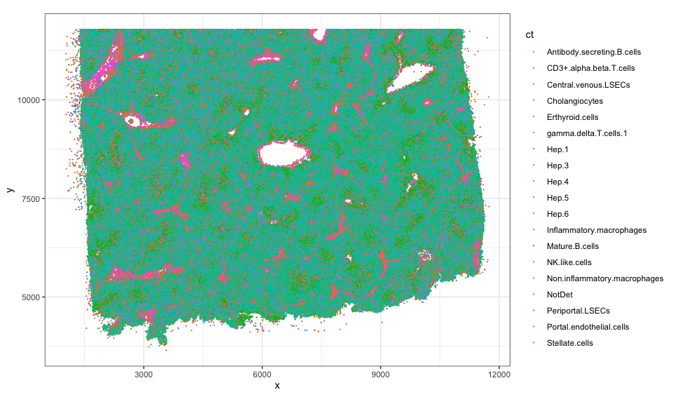
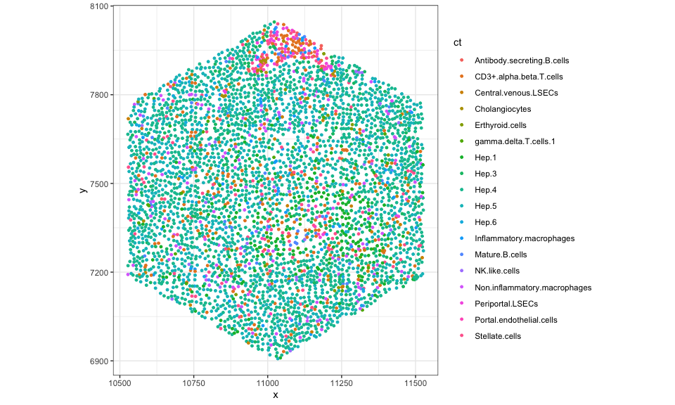
Let’s use ggplot2 to visualize these cell-type annotations in this
tissue section. From this, we can appreciate that this tissue section is
roughly 10mm by 12mm (10000um by 12000um) with ~300k cells comprising
19 cell-types.
length(ct)
## [1] 332877
length(levels(ct))
## [1] 19
## plot
suppressMessages(library(ggplot2))
df <- data.frame(pos, ct = ct)
ggplot(df, aes(x = x, y = y, color = ct)) +
  coord_fixed() +
  geom_point(size = 0.001) +
  theme_bw()
 If we
estimate the cell-type proportions from this whole tissue, we can
appreciate that roughly 38% of the cells are
If we
estimate the cell-type proportions from this whole tissue, we can
appreciate that roughly 38% of the cells are Hep.4 cells, 5% are
Stellate.cells, 4% are CD3+.alpha.beta.T.cells cells, 2% are
Inflammatory.macrophages and so forth.
## count number of each cell-type, divide by total cells
## and multiply by 100 to make into percents
globalEstimate <- table(ct)/length(ct)*100
sort(globalEstimate)
## ct
##                       NotDet     Portal.endothelial.cells
##                  0.001201645                  0.161320848
##              Erthyroid.cells   Antibody.secreting.B.cells
##                  0.313629359                  0.424481115
##                NK.like.cells               Mature.B.cells
##                  0.826731796                  0.879604178
##        gamma.delta.T.cells.1         Central.venous.LSECs
##                  0.955608228                  1.326616137
##               Cholangiocytes     Inflammatory.macrophages
##                  1.436867071                  1.767019049
##             Periportal.LSECs                        Hep.6
##                  1.827401713                  1.857442839
## Non.inflammatory.macrophages      CD3+.alpha.beta.T.cells
##                  2.870730029                  4.104819498
##               Stellate.cells                        Hep.1
##                  4.951378437                  5.216341171
##                        Hep.3                        Hep.5
##                  6.390949209                 26.836939771
##                        Hep.4
##                 37.850917907
Using SEraster to create spatial bootstrap samples
However, what if we didn’t have a large 10mm by 12mm tissue section? What if I had a tiny roughly 1mm by 1mm (1000um by 1000um) tissue section? How different would my cell-type proportion estimates be in that case?
Let’s use SEraster to help us find out. I will follow the SEraster
tutorials
to convert my cell positions matrix pos and cell-type annotations
vector ct into a SpatialExperiment object and then use SEraster to
aggregate the cell information into non-overlapping, spatially
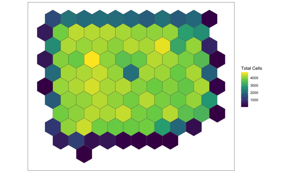
contiguous, hexagonal pixels that are 1000um wide. We can plot the
results to appreciate the size of the new hexagonal pixels and the
number of cells per pixel.
suppressMessages(library(SpatialExperiment))
suppressMessages(library(SEraster))

## convert to SE object
spe <- SpatialExperiment::SpatialExperiment(
  spatialCoords = as.matrix(pos),
  colData = data.frame(ct=ct)
)

## rasterize at 1000um resolution with hexagons
rastCt <- SEraster::rasterizeCellType(spe,
                                      col_name = "ct",
                                      resolution = 1000,
                                      fun = "sum",
                                      square = FALSE)

## plot
SEraster::plotRaster(rastCt, name = "Total Cells")
## Coordinate system already present. Adding new coordinate system, which will
## replace the existing one.
Note that SEraster outputs a SpatialExperiment object. Let’s take a
closer look at the colData slot of this object.
class(rastCt)
## [1] "SpatialExperiment"
## attr(,"package")
## [1] "SpatialExperiment"
head(colData(rastCt))
## DataFrame with 6 rows and 6 columns
##          num_cell                             cellID_list        type
##         <integer>                                  <list> <character>
## pixel15        30   c_1_169_110,c_1_169_35,c_1_148_40,...     hexagon
## pixel16       412    c_1_85_255,c_1_85_93,c_1_106_108,...     hexagon
## pixel17       515     c_1_22_152,c_1_22_275,c_1_22_85,...     hexagon
## pixel20      1041 c_1_250_650,c_1_250_852,c_1_270_204,...     hexagon
## pixel21      1749 c_1_190_370,c_1_190_533,c_1_190_633,...     hexagon
## pixel22      2016 c_1_107_810,c_1_107_954,c_1_127_117,...     hexagon
##         resolution               geometry   sample_id
##          <numeric>          <sfc_POLYGON> <character>
## pixel15       1000 list(c(1027, 527, 52..    sample01
## pixel16       1000 list(c(1027, 527, 52..    sample01
## pixel17       1000 list(c(1027, 527, 52..    sample01
## pixel20       1000 list(c(1527, 1027, 1..    sample01
## pixel21       1000 list(c(1527, 1027, 1..    sample01
## pixel22       1000 list(c(1527, 1027, 1..    sample01
We can see that SEraster has kept track of the number of cells in each
of these hexagonal pixels as well as the names of the cells per pixel.
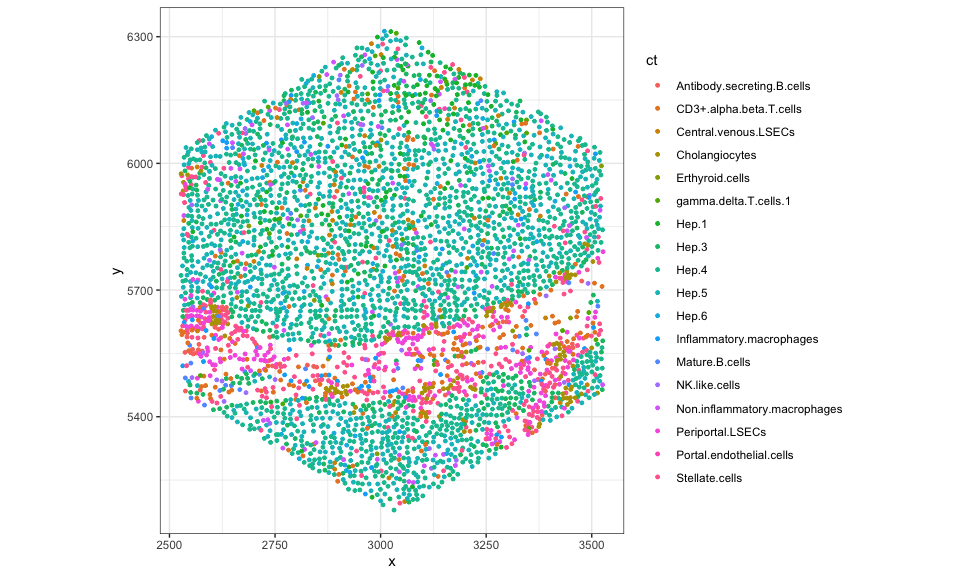
Let’s grab the names of the cells for a few pixels and plot them in the
tissue.
## 20th pixel
cells <- colData(rastCt)$cellID_list[[20]]
## visualize just the cells in this hexagonal pixel
dfsub <- data.frame(pos[cells,], ct = ct[cells])
ggplot(dfsub, aes(x = x, y = y, color = ct)) +
  coord_fixed() +
  geom_point(size = 1) +
  theme_bw()
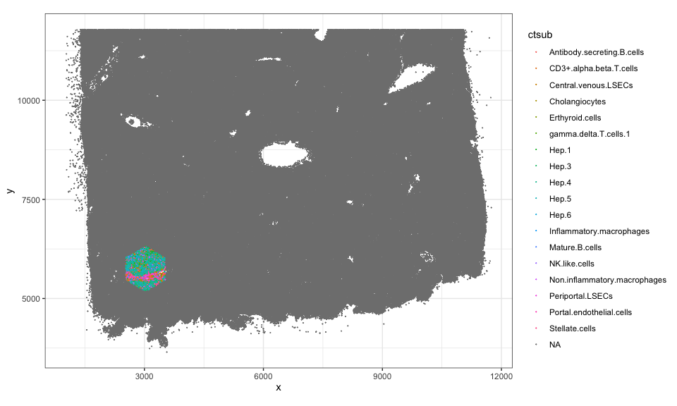
## in whole tissue by setting cells not in hexagonal to NA
ctsub <- ct
ctsub[!(names(ctsub) %in% cells)] <- NA
df <- data.frame(pos, ctsub = ctsub)
ggplot(df, aes(x = x, y = y, color = ctsub)) +
  coord_fixed() +
  geom_point(size = 0.001) +
  theme_bw()
## 100th pixel
cells <- colData(rastCt)$cellID_list[[100]]
## visualize just the cells in this hexagonal pixel
df <- data.frame(pos[cells,], ct = ct[cells])
ggplot(df, aes(x = x, y = y, color = ct)) +
  coord_fixed() +
  geom_point(size = 1) +
  theme_bw()
## in whole tissue by setting cells not in hexagonal to NA
ctsub <- ct
ctsub[!(names(ctsub) %in% cells)] <- NA
df <- data.frame(pos, ctsub = ctsub)
ggplot(df, aes(x = x, y = y, color = ctsub)) +
  coord_fixed() +
  geom_point(size = 0.001) +
  theme_bw()
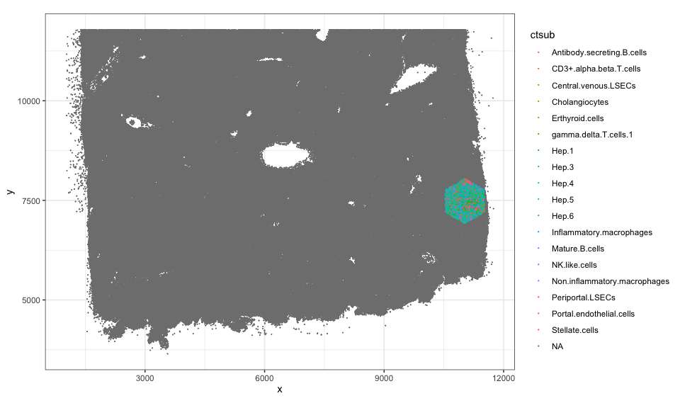
Note we have 109 such pixels.
length(colData(rastCt)$cellID_list)
## [1] 109
Using spatial bootstraps to evaluate stability of cell-type proportions
So let’s see what happens if we estimate the cell-type proportion using just the cells in each hexagonal pixel.
## grab list cell IDs for each hexagonal pixel
cellidsPerBiopsy <- colData(rastCt)$cellID_list
names(cellidsPerBiopsy) <- colnames(rastCt)

## loop through and count number of each cell-type
ctprop <- do.call(rbind, lapply(cellidsPerBiopsy, function(i) {
  table(ct[i])
}))
rownames(ctprop) <- names(cellidsPerBiopsy)
head(ctprop)
##         Antibody.secreting.B.cells CD3+.alpha.beta.T.cells Central.venous.LSECs
## pixel15                          0                      17                    0
## pixel16                          0                      34                    5
## pixel17                          0                      48                    5
## pixel20                          2                      58                   15
## pixel21                          0                      64                   24
## pixel22                          1                     114                   26
##         Cholangiocytes Erthyroid.cells gamma.delta.T.cells.1 Hep.1 Hep.3 Hep.4
## pixel15              0               1                     0     0     0     0
## pixel16              9               0                     9     4    22   152
## pixel17              3               1                    12     4    25   197
## pixel20             29               2                     7   154    62   372
## pixel21             22               2                    12   233   101   621
## pixel22              3               4                    21   107   121   857
##         Hep.5 Hep.6 Inflammatory.macrophages Mature.B.cells NK.like.cells
## pixel15     0     0                        3              5             4
## pixel16   116     5                        6              5            10
## pixel17   152     7                        9             14             7
## pixel20   226     6                        6             11             9
## pixel21   492    21                       17             20            13
## pixel22   525    26                       35             21            31
##         Non.inflammatory.macrophages NotDet Periportal.LSECs
## pixel15                            0      0                0
## pixel16                           17      0                4
## pixel17                           18      0                0
## pixel20                           25      0                5
## pixel21                           41      1                1
## pixel22                           64      0                3
##         Portal.endothelial.cells Stellate.cells
## pixel15                        0              0
## pixel16                        2             12
## pixel17                        0             13
## pixel20                        5             47
## pixel21                        2             62
## pixel22                        3             54
## divide by total cells per pixel
## and multiple by 100 to make into percents
ctpropNorm <- ctprop/rowSums(ctprop)*100
head(rowSums(ctpropNorm)) ## confirm sum is 100
## pixel15 pixel16 pixel17 pixel20 pixel21 pixel22
##     100     100     100     100     100     100
head(ctpropNorm)
##         Antibody.secreting.B.cells CD3+.alpha.beta.T.cells Central.venous.LSECs
## pixel15                 0.00000000               56.666667            0.0000000
## pixel16                 0.00000000                8.252427            1.2135922
## pixel17                 0.00000000                9.320388            0.9708738
## pixel20                 0.19212296                5.571566            1.4409222
## pixel21                 0.00000000                3.659234            1.3722127
## pixel22                 0.04960317                5.654762            1.2896825
##         Cholangiocytes Erthyroid.cells gamma.delta.T.cells.1      Hep.1
## pixel15      0.0000000       3.3333333             0.0000000  0.0000000
## pixel16      2.1844660       0.0000000             2.1844660  0.9708738
## pixel17      0.5825243       0.1941748             2.3300971  0.7766990
## pixel20      2.7857829       0.1921230             0.6724304 14.7934678
## pixel21      1.2578616       0.1143511             0.6861063 13.3218982
## pixel22      0.1488095       0.1984127             1.0416667  5.3075397
##            Hep.3    Hep.4    Hep.5     Hep.6 Inflammatory.macrophages
## pixel15 0.000000  0.00000  0.00000 0.0000000               10.0000000
## pixel16 5.339806 36.89320 28.15534 1.2135922                1.4563107
## pixel17 4.854369 38.25243 29.51456 1.3592233                1.7475728
## pixel20 5.955812 35.73487 21.70989 0.5763689                0.5763689
## pixel21 5.774728 35.50600 28.13036 1.2006861                0.9719840
## pixel22 6.001984 42.50992 26.04167 1.2896825                1.7361111
##         Mature.B.cells NK.like.cells Non.inflammatory.macrophages     NotDet
## pixel15      16.666667    13.3333333                     0.000000 0.00000000
## pixel16       1.213592     2.4271845                     4.126214 0.00000000
## pixel17       2.718447     1.3592233                     3.495146 0.00000000
## pixel20       1.056676     0.8645533                     2.401537 0.00000000
## pixel21       1.143511     0.7432819                     2.344197 0.05717553
## pixel22       1.041667     1.5376984                     3.174603 0.00000000
##         Periportal.LSECs Portal.endothelial.cells Stellate.cells
## pixel15       0.00000000                0.0000000       0.000000
## pixel16       0.97087379                0.4854369       2.912621
## pixel17       0.00000000                0.0000000       2.524272
## pixel20       0.48030740                0.4803074       4.514890
## pixel21       0.05717553                0.1143511       3.544883
## pixel22       0.14880952                0.1488095       2.678571
And let’s visualize the resulting cell-type proportions per hexagonal pixel as a stacked barplot.
suppressMessages(library(reshape2))

# Melt the data frame to long format
df <- data.frame(ctpropNorm)
df$Sample <- rownames(df)
dfLong <- melt(df, id.vars = "Sample", variable.name = "CellType", value.name = "Proportion")
head(dfLong)
##    Sample                   CellType Proportion
## 1 pixel15 Antibody.secreting.B.cells 0.00000000
## 2 pixel16 Antibody.secreting.B.cells 0.00000000
## 3 pixel17 Antibody.secreting.B.cells 0.00000000
## 4 pixel20 Antibody.secreting.B.cells 0.19212296
## 5 pixel21 Antibody.secreting.B.cells 0.00000000
## 6 pixel22 Antibody.secreting.B.cells 0.04960317
# Create the stacked barplot using ggplot2
ggplot(dfLong, aes(x = Sample, y = Proportion, fill = CellType)) +
  geom_bar(stat = "identity") +
  labs(title = "Stacked Barplot of Cell Type Proportions",
       x = "Sample",
       y = "Proportion") +
  theme_minimal() +
  theme(axis.text.x = element_text(angle = 90, vjust = 0.5, hjust=1, size=5))
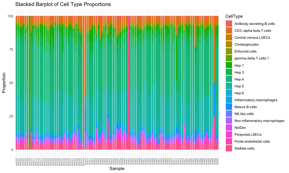
There are definitely some hexagonal pixels that have very distinct cell-type proportions. Let’s see which ones are the most different from our global cell-type proportion estimate.
diff <- sapply(1:nrow(ctpropNorm), function(i) {
  sum((ctpropNorm[i,]-globalEstimate)^2)
})
names(diff) <- rownames(ctpropNorm)

head(sort(diff, decreasing=TRUE))
##  pixel109  pixel148   pixel43   pixel15   pixel97   pixel73
## 12095.864 11466.022 11296.710  5510.753  4223.865  1688.273
Indeed, it looks like our estimate of cell-type proportions is quite
different for this pixel109 compared to original global estimate. In
pixel109, 100% of the cells are of the gamma.delta.T.cells.1
cell-type! However, if we look closer, it seems like this hexagonal
pixel only has 1 cell in it!
ctpropNorm['pixel109',]
##   Antibody.secreting.B.cells      CD3+.alpha.beta.T.cells
##                            0                            0
##         Central.venous.LSECs               Cholangiocytes
##                            0                            0
##              Erthyroid.cells        gamma.delta.T.cells.1
##                            0                          100
##                        Hep.1                        Hep.3
##                            0                            0
##                        Hep.4                        Hep.5
##                            0                            0
##                        Hep.6     Inflammatory.macrophages
##                            0                            0
##               Mature.B.cells                NK.like.cells
##                            0                            0
## Non.inflammatory.macrophages                       NotDet
##                            0                            0
##             Periportal.LSECs     Portal.endothelial.cells
##                            0                            0
##               Stellate.cells
##                            0
colData(rastCt)['pixel109',]
## DataFrame with 1 row and 6 columns
##           num_cell cellID_list        type resolution               geometry
##          <integer>      <list> <character>  <numeric>          <sfc_POLYGON>
## pixel109         1  c_1_301_25     hexagon       1000 list(c(9027, 8527, 8..
##            sample_id
##          <character>
## pixel109    sample01
## plot pixel109
cells <- colData(rastCt)$cellID_list[[109]]
## visualize just the cells in this hexagonal pixel
df <- data.frame(pos[cells,], ct = ct[cells])
ggplot(df, aes(x = x, y = y, color = ct)) +
  coord_fixed() +
  geom_point(size = 1) +
  theme_bw()
![]()
## in whole tissue by setting cells not in hexagonal to NA
ctsub <- ct
ctsub[!(names(ctsub) %in% cells)] <- NA
df <- data.frame(pos, ctsub = ctsub)
ggplot(df, aes(x = x, y = y, color = ctsub)) +
  coord_fixed() +
  geom_point(size = 0.001) +
  theme_bw()
![]()
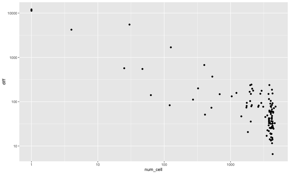
If we look at the total number of cells per hexagonal pixel versus how different their cell-type proportion estimate is from the global estimate, we definitely see an association where pixels with very few cells are more different in their estimates as expected. These pixels are likely towards the edge of the tissue and therefore not very representative.
df <- data.frame(num_cell = colData(rastCt)$num_cell, diff = diff)
## note we are plotting on a log scale!
ggplot(df, aes(x=num_cell, y=diff)) + geom_point() + scale_x_log10() + scale_y_log10()
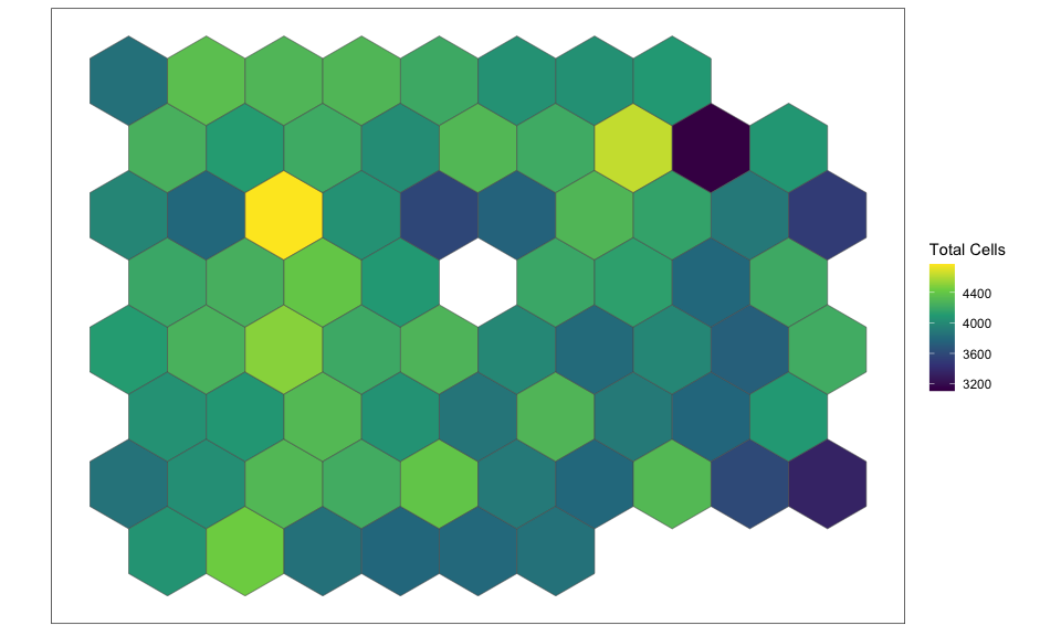
If we restrict to hexagonal pixels with more than 3000 cells, we can confirm these pixels are not on the edge of the tissue section.
## histogram of number of cells per pixel
hist(colData(rastCt)$num_cell)
abline(v = 3000, col='red')
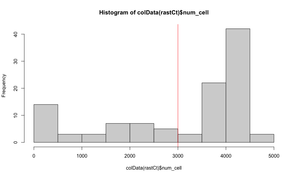
## get pixels with more than 3000 cells
goodPixels <- colnames(rastCt)[colData(rastCt)$num_cell > 3000]
length(goodPixels)
## [1] 70
head(goodPixels)
## [1] "pixel26" "pixel27" "pixel28" "pixel29" "pixel32" "pixel33"
SEraster::plotRaster(rastCt[, goodPixels], name = "Total Cells")
## Coordinate system already present. Adding new coordinate system, which will
## replace the existing one.
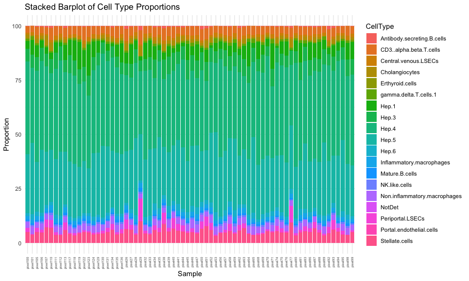
And now, we can see a pretty consistent cell-type proportion distribution compared to our original global estimate.
## just look at ctpropNorm for good pixels
df <- data.frame(ctpropNorm[goodPixels,])
df$Sample <- rownames(df)
dfLong <- melt(df, id.vars = "Sample", variable.name = "CellType", value.name = "Proportion")
ggplot(dfLong, aes(x = Sample, y = Proportion, fill = CellType)) +
  geom_bar(stat = "identity") +
  labs(title = "Stacked Barplot of Cell Type Proportions",
       x = "Sample",
       y = "Proportion") +
  theme_minimal() +
  theme(axis.text.x = element_text(angle = 90, vjust = 0.5, hjust=1, size=5))
We can even focus on just one cell-type, for example the
Stellate.cells, and fit a gaussian distribution to all the estimates
of this cell-type’s proportional representation across all of our
hexagonal pixels.
cct <- 'Stellate.cells'
cellProportions <- ctpropNorm[goodPixels,cct]

df <- data.frame(x = cellProportions)

# Fit Gaussian distribution
mu <- mean(cellProportions)
sigma <- sd(cellProportions)
x <- seq(0, 25, length.out = 100) # fit from 0 to 25%
y <- dnorm(x, mean = mu, sd = sigma)
fit <- data.frame(x = x, y = y)

# Add Gaussian distribution line to the plot
ggplot(df, aes(x = x)) +
  geom_histogram(binwidth = 0.02, color = "black") +
  labs(title = paste0("Estimate of ", cct, " Cell-Type Proportion\nin the Liver from 100um Hexagonal Pixels"),
       x = paste0(cct, " Cell-Type Proportion"),
       y = "Frequency") +
  theme_minimal() +
  geom_line(data = fit, aes(x = x, y = y), color = "red", linewidth = 1)
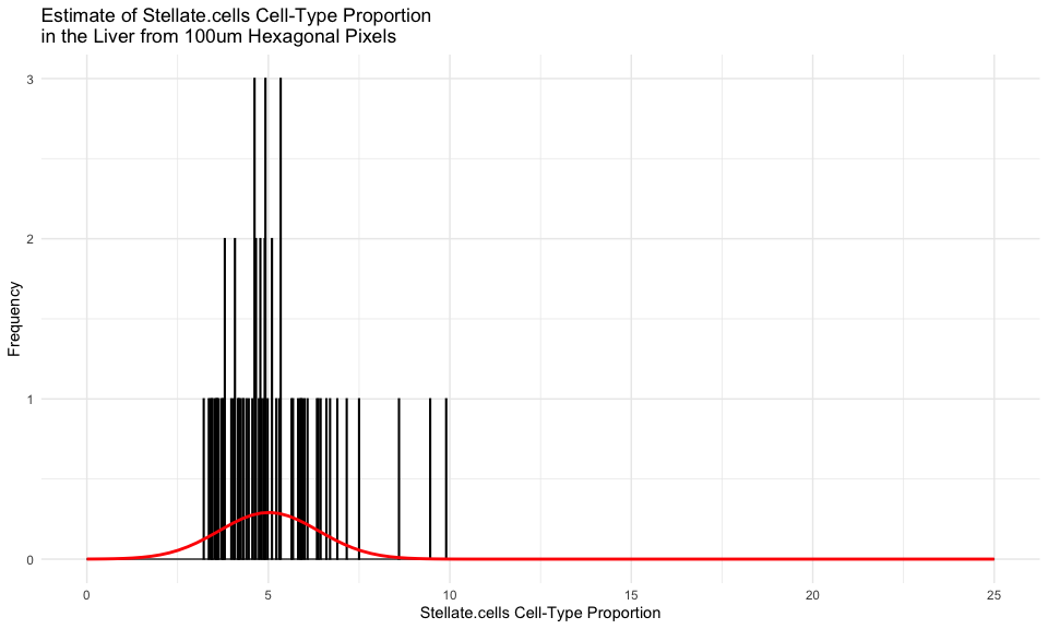
According to Wikipedia, which cites this paper, “in normal liver…stellate cells represent 5-8% of the total number of liver cells.” So it seems like our estimate is pretty consistent!
Of course while this type of spatial bootstrapping does not account for inter-patient variability or other technical and biological variation that may contribute to cell-type proportion variability, it can give us a sense for the degree of intra-sample cell-type proportion variability for tissue sections of a particular size, in this case 1000um.
Try it out for yourself!
- If you choose a square pixel instead of hexagonal by setting
square = TRUE, how do the results change? - If you choose a smaller (or larger) hexagonal pixel size, how do the results change?
- Calculate another statistic per pixel such as cell-type spatial colocalization relationships and evaluate its stability.
- Apply what you’ve learned towards your own spatial omics data analysis.
Recent Posts
- The Mentorship Index on 01 March 2026
- Vibe coding with SEraster and STcompare to compare spatial transcriptomics technologies on 22 February 2026
- RNA velocity in situ infers gene expression dynamics using spatial transcriptomics data on 13 October 2025
- Analyzing ICE Arrest Data - Part 2 on 27 September 2025
- Analyzing ICE Detention Data from 2021 to 2025 on 10 July 2025