Aligning fluorescence and histological images from the same tissue section at single-cell resolution with STalign

Computational methods frequently apply mathematical models tailored to address specific problems. In our recent paper “STalign: Alignment of spatial transcriptomics data using diffeomorphic metric mapping”, we presented a computational method called STalign that builds on the mathematics of large deformation diffeomorphic metric mapping (LDDMM) to structurally align spatial transcriptomics data. In our paper as well as via various tutorials, we demonstrate how to structurally align:

• two MERFISH spatial transcriptomics datasets of corodonal sections of the mouse brain from different animals
• two Xenium spatial transcriptomics datasets of partially matched serials section from breast cancer
• a MERFISH dataset to a Visium dataset of the mouse brain from different animals
• and more

However, by understanding the mathematical underpinnings of these computational methods, we can often extrapolate their uses beyond initially envisioned applications. As such, we can often use computational methods for a different problem that the original authors didn’t think of (or at least didn’t describe). In this blog post, I will demonstrate how to use STalign to align a fluorescence and histological image from the same tissue. Unlike previously demonstrations that have focused on either tissue sections from different animals or serial sections where perfect single-cell resolution matching is not possible, here, we will focus on aligning two images from different modalities of the same tissue at single-cell resolution.

Simulating images for alignment

For the purposes of this demonstration, I will simulate two images of lung tissue using this H&E image taken from Wikipedia. I will invert and greyscale to simulate what I might get if I subjected the tissue to some type of fluorescence imaging. I will also crop and zoom a little for the H&E image to simulate how different imaging modalities may often capture different extents of the tissue. I could also rotate or distort the images further to simulate common transformations induced during the data collection process, but that will be left as an exercise to the students.

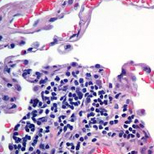
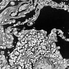
The general idea is to create two tissue images that I know can be aligned perfectly at single cell resolution but to also induce transformations that make the alignment problem slightly more difficult and similar to a real-life scenario. If we can align these simulated partially-matched fluorescence and H&E images, then we have a chance at aligning real partially-matched fluorescence and H&E images taken from the same tissue in the future.

Processing images for STalign

I have already installed STalign and its associated dependencies so I will use a jupyter notebook to run the following Python code.

from STalign import STalign
import matplotlib.pyplot as plt
import numpy as np
import torch

To get started, I will read in the images and visualize them using matplotlib. We will refer to these as our source and our target images. Simply overlaying these images highlights how they are not aligned. Our goal is to find a transformation that when applied to our source, makes it aligned with our target, ideally at single-cell resolution.

## source
image_file = 'cells2_crop.jpg'
G = plt.imread(image_file)

## target
image_file = 'cells.jpg'
V = plt.imread(image_file)

## plot
fig,ax = plt.subplots(1,3)
ax[0].imshow(V) 
ax[1].imshow(G) 
ax[2].imshow(V)
ax[2].imshow(G, alpha=0.5)
ax[0].set_title('source', fontsize=15)
ax[1].set_title('target', fontsize=15)
ax[2].set_title('combined', fontsize=15)
plt.show()

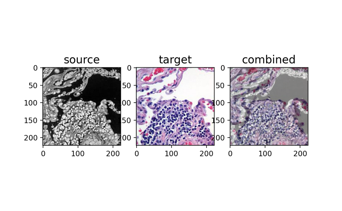
Note that these images are 223x223 pixels with 3 channels (red, green, blue) resulting in a matrix representation that is 223x223x3. The numeric values in these 3 channels also can be as large as 252 and 255 respectively.

print(V.shape)
print(G.shape)
print([V.min(), V.max()])
print([G.min(), G.max()])

(223, 223, 3)
(223, 223, 3)
[0, 252]
[0, 255]

As a first step, we will normalize these images, which just means making their numeric values range from 0 to 1.

Inorm = STalign.normalize(V)
Jnorm = STalign.normalize(G)

print(Inorm.shape)
print(Jnorm.shape)
print([Inorm.min(), Inorm.max()])
print([Jnorm.min(), Jnorm.max()])

(223, 223, 3)
(223, 223, 3)
[0.0, 1.0]
[0.0, 1.0]

Note this does not change the general appearance of the images, just the range of intensity values. You can visualize the resulting normalized images to prove this for yourself.

fig,ax = plt.subplots(1,3)
ax[0].imshow(Inorm) 
ax[1].imshow(Jnorm) 
ax[2].imshow(Inorm)
ax[2].imshow(Jnorm, alpha=0.5)
ax[0].set_title('source \n normalized', fontsize=15)
ax[1].set_title('target \n normalized', fontsize=15)
ax[2].set_title('combined', fontsize=15)
plt.show()

Landmark-based affine transformation with STalign

As a point of comparison, we will first perform a landmark-based affine transformation. I will manually place some points that visually corresponds to matched landmarks in my source and target images. As such, if I am able to find a transformation that when applied to the landmark points in our source, minimizes the distance with corresponding landmark points in our target, I can apply the transformation to align my source and target images.

## manually make very approximate landmark points 
## important: points must be in y,x for torch later
pointsI = np.array([[150, 190], [100, 60], [75, 100]])
pointsJ = np.array([[160, 200], [100, 50], [75, 100]])

## plot
fig,ax = plt.subplots(1,2)
ax[0].imshow(Inorm)
ax[1].imshow(Jnorm)
ax[0].scatter(pointsI[:,1],pointsI[:,0], c='red')
ax[1].scatter(pointsJ[:,1],pointsJ[:,0], c='red')
for i in range(pointsI.shape[0]):
    ax[0].text(pointsI[i,1],pointsI[i,0],f'{i}', c='red')
    ax[1].text(pointsJ[i,1],pointsJ[i,0],f'{i}', c='red')
plt.show()

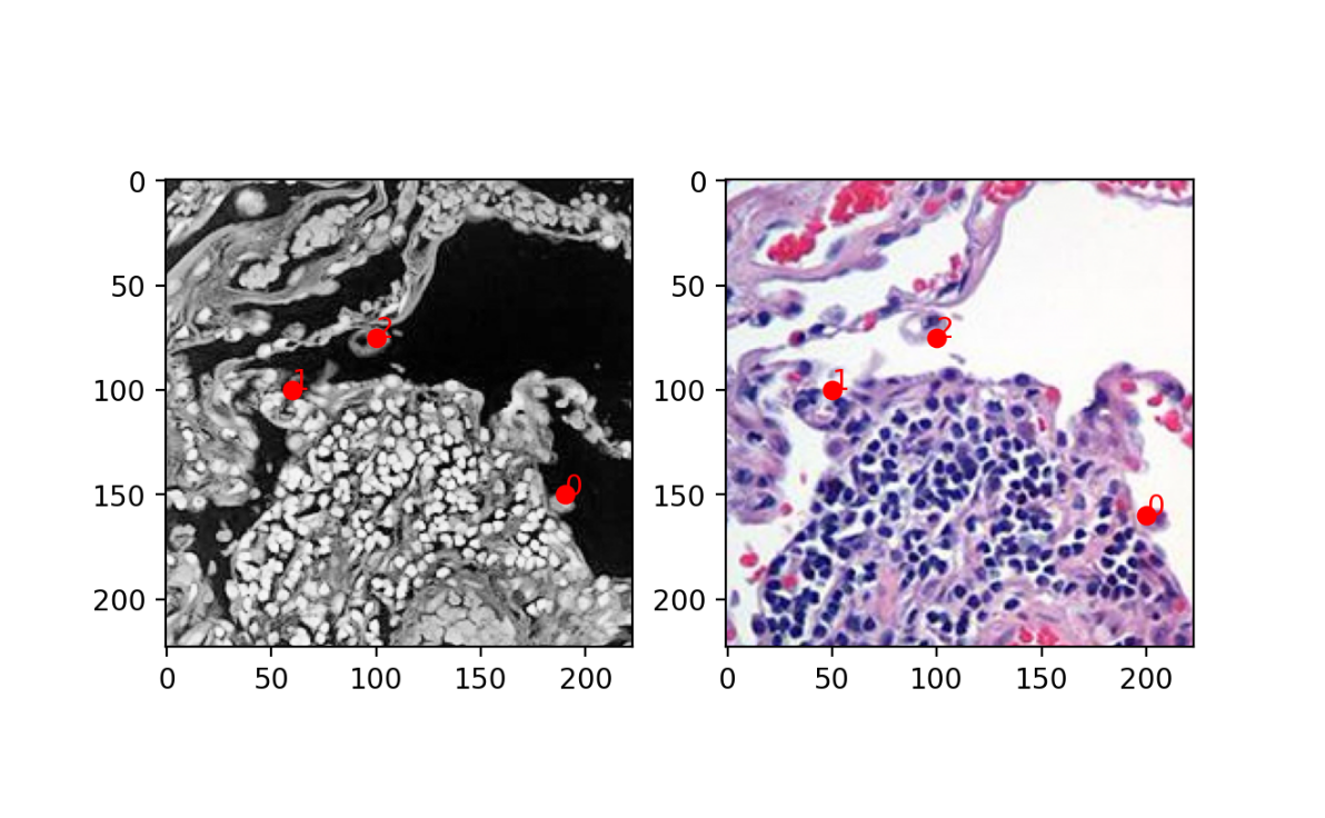
As you can see, I did not do a perfect job. It will be left as an exercise for the student to improve upon my landmarks and see if that changes your alignment performance. But for now, I will use STalign to perform an affine transformation by minimizing the distance between these manually placed landmarks.

## compute initial affine transformation from points
L,T = STalign.L_T_from_points(pointsI, pointsJ)
A = STalign.to_A(torch.tensor(L),torch.tensor(T))
print(A)
print(A.shape)

tensor([[  1.0762,   0.0476, -10.4762],
        [ -0.0952,   1.1905, -11.9048],
        [  0.0000,   0.0000,   1.0000]], dtype=torch.float64)
torch.Size([3, 3])

Note the resulting A matrix is a 3x3 tensor representing our learned affine transformation.

Now we can apply the affine transformation to our original source image. Note, STalign uses pytorch for learning and applying transformation, which requires converting our image represented as a matrix into a tensor, which requires transposing our matrix. Note that the input tensor dimensions are 3x223x223 now.

# transpose matrices into right dimensions for torch later, set up extent
I = Inorm.transpose(2,0,1)
print(I.shape)
YI = np.array(range(I.shape[1]))*1. 
XI = np.array(range(I.shape[2]))*1. 
extentI = STalign.extent_from_x((YI,XI))

J = Jnorm.transpose(2,0,1)
print(J.shape)
YJ = np.array(range(J.shape[1]))*1. 
XJ = np.array(range(J.shape[2]))*1. 
extentJ = STalign.extent_from_x((YJ,XJ))

(3, 223, 223)
(3, 223, 223)

After applying the affine transformation, we can convert the output back into a 223x223x3 matrix to be able to visualize the results using matplotlib.

## Apply transformation to original image
AI = STalign.transform_image_source_with_A(A, [YI,XI], I, [YJ,XJ])
Iaffine = AI.permute(1,2,0).numpy() ## convert from torch coordinates back to image matrix

print(I.shape)
print(AI.shape)
print(Iaffine.shape)

(3, 223, 223)
torch.Size([3, 223, 223])
(223, 223, 3)

fig,ax = plt.subplots(1,3)
ax[0].imshow(Iaffine) 
ax[1].imshow(Jnorm) 
ax[2].imshow(Iaffine)
ax[2].imshow(Jnorm, alpha=0.5)
ax[0].set_title('source \n with affine \n transform', fontsize=15)
ax[1].set_title('target', fontsize=15)
ax[2].set_title('combined', fontsize=15)
plt.show()

As we can see, the landmark-based affine transformation is not perfect; we do not get single-cell resolution corresponendence between the two images. Perhaps I could have placed my landmarks a bit better, but in general, we are limited in our ability to place landmarks perfectly, so there will likely always be some degree of imperfection using this approach.

Automated alignment by affine and LDDMM with STalign

So we will instead seek to use a gradient descent to minimize a specific error function that captures the disimilarity between the source and target image subject to regularization constraints:

Consult the original publication for more details.

From the objective function, there are a number of hyperparameters we can tune. As described in the STalign documentation, epV is our gradient descent step size. Because I want to align at single-cell resolution, I will choose a very small step size to make sure I don’t overshoot.

I will also change a, the smoothness scale of velocity field, to be smaller to match the size of my actual image. Note that since my image is only 223x223 pixels, if I choose an a that is way too big, the resulting transformation will effectively be rigid. If a choose an a that is too small, I could induce very small local diffeomorphisms that should not be necessary.

I will run the gradient descent for 1000 iterations via ‘niter’ and use the learned affine transformation components L and T to initialize our alignment. It will be left as an exercise to the student to try different hypermaraters to see how it impacts the alignment.

torch.set_default_device('cpu')
device = 'cpu'

# keep all other parameters default
params = {'L':L,'T':T,
       'niter':1000,
       'device':device,
       'a':50,
       'epV':1
}

## run LDDMM
out = STalign.LDDMM([YI,XI],I,[YJ,XJ],J,**params)
plt.show()

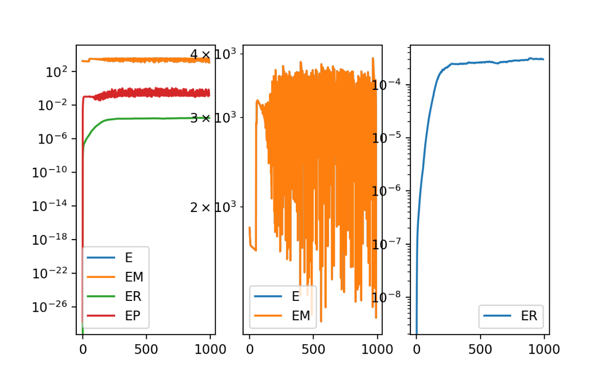
Looking at the resulting error as a function of iterations in the gradient descent, we can see the regularization term ER plateauing but the matching term EM is oddly fluctuating. This suggests we are not at a stable solution. But we will march forward and visualize the results anyway.

## get necessary output variables
A = out['A']
v = out['v']
xv = out['xv']

We will apply the learned transformation to phi to the original source image (again careful with your matrix versus tensor dimensions) and visualize the results.

# build transformation
phii = STalign.build_transform(xv,v,A,XJ=[YJ,XJ],direction='b')
# apply transformation to Iorig
Iorig = STalign.normalize(V)
Iorig = Iorig.transpose(2,0,1) # convert to [3, 223, 223] tensor 
phiI = STalign.transform_image_source_to_target(xv,v,A,[YI,XI],Iorig,[YJ,XJ])
phiI = phiI.permute(1,2,0).numpy() # convert to [223, 223, 3] numpy matrix for plotting

# plot
fig,ax = plt.subplots(1,3)
ax[0].imshow(phiI)
ax[1].imshow(Jnorm)
ax[2].imshow(phiI)
ax[2].imshow(Jnorm, alpha=0.5)
ax[0].set_title('source with \nLDDMM \ntransform', fontsize=15)
ax[1].set_title('target', fontsize=15)
ax[2].set_title('combined', fontsize=15)
plt.show()

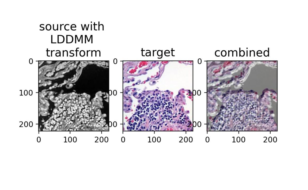
Hum, this is not great either! What’s going on? Perhaps it is because we are not at a stable solution. If we run for additional iterations, could we converge onto a more stable solution? Maybe our gradient descent step size is too big? Maybe we should tinker with other parameters?

There are many things we can try, but in this case, by understanding the mathematical underpinnings, we can figure out the “correct” approach much more quickly.

Creating a smooth image representation for STalign

In the original publication, STalign was applied to single-cell resolution ST technologies where both the source and target ST datasets are represented as (x,y) coordinates of cellular positions. Solving the alignment with respect to single cells has quadratic complexity and is computationally intractable, so STalign applies a rasterization approach that models the single cell positions as a marginal space measure that is convolved with a Gaussian kernel to obtain the smooth image. This smooth image representation is useful in the gradient descent for learning the transformation that can then be applied back to the original source cellular positions to achieve alignment with the target.

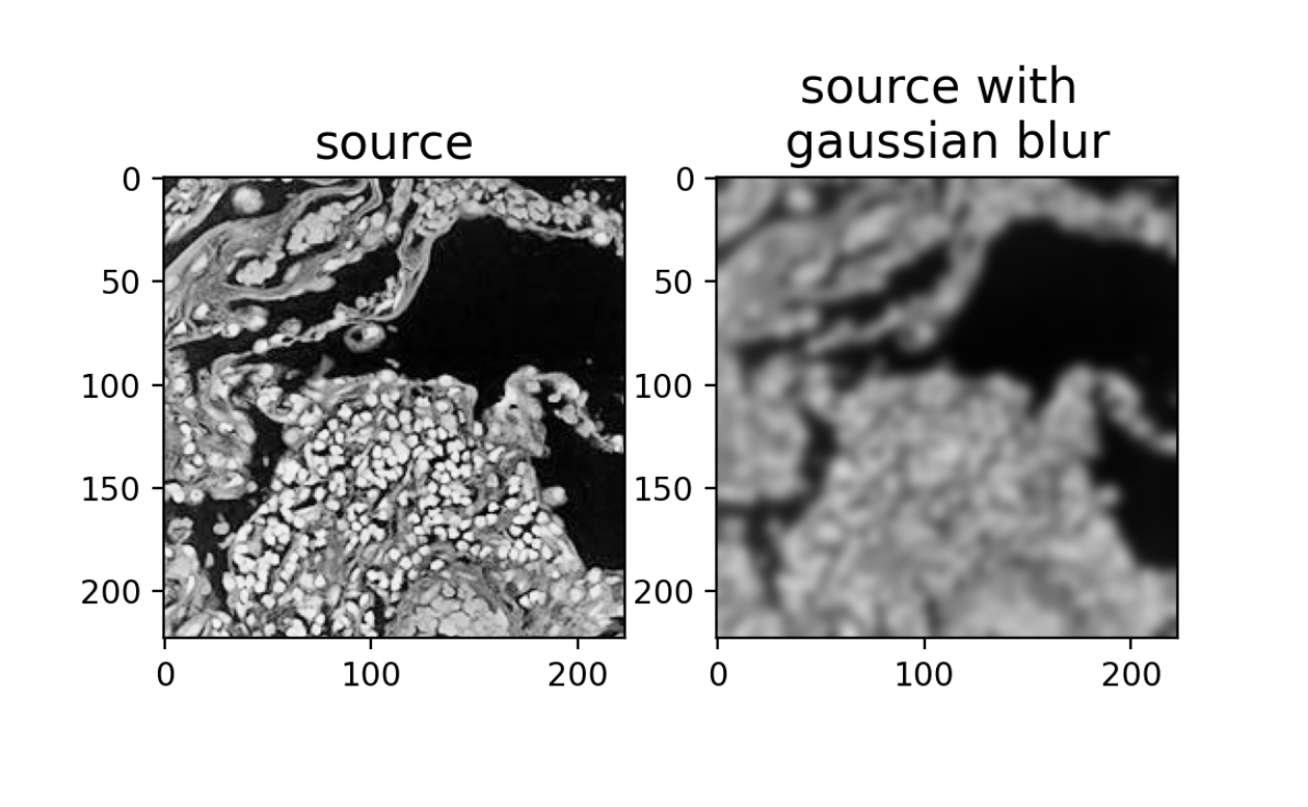
Here, we are starting with an image instead of cellular positions. But we can still create a “smooth image representation” by convolving with our own Gaussian kernel. I will simply apply a Gaussian filter to effectively blur the intensities for our source image.

from scipy.ndimage import gaussian_filter

V2 = gaussian_filter(V, sigma=3)

fig,ax = plt.subplots(1,2)
ax[0].imshow(V)
ax[1].imshow(V2)
ax[0].set_title('source', fontsize=15)
ax[1].set_title('source with \ngaussian blur', fontsize=15)
plt.show()

Now let’s try to run the automated alignment by affine and LDDMM on the source image with Gaussian blur instead.

# use source with gaussian blur to learn phii
Iblurnorm = STalign.normalize(V2)
Iblur = Iblurnorm.transpose(2,0,1)

# run LDDMM
out = STalign.LDDMM([YI,XI],Iblur,[YJ,XJ],J,**params)
plt.show()

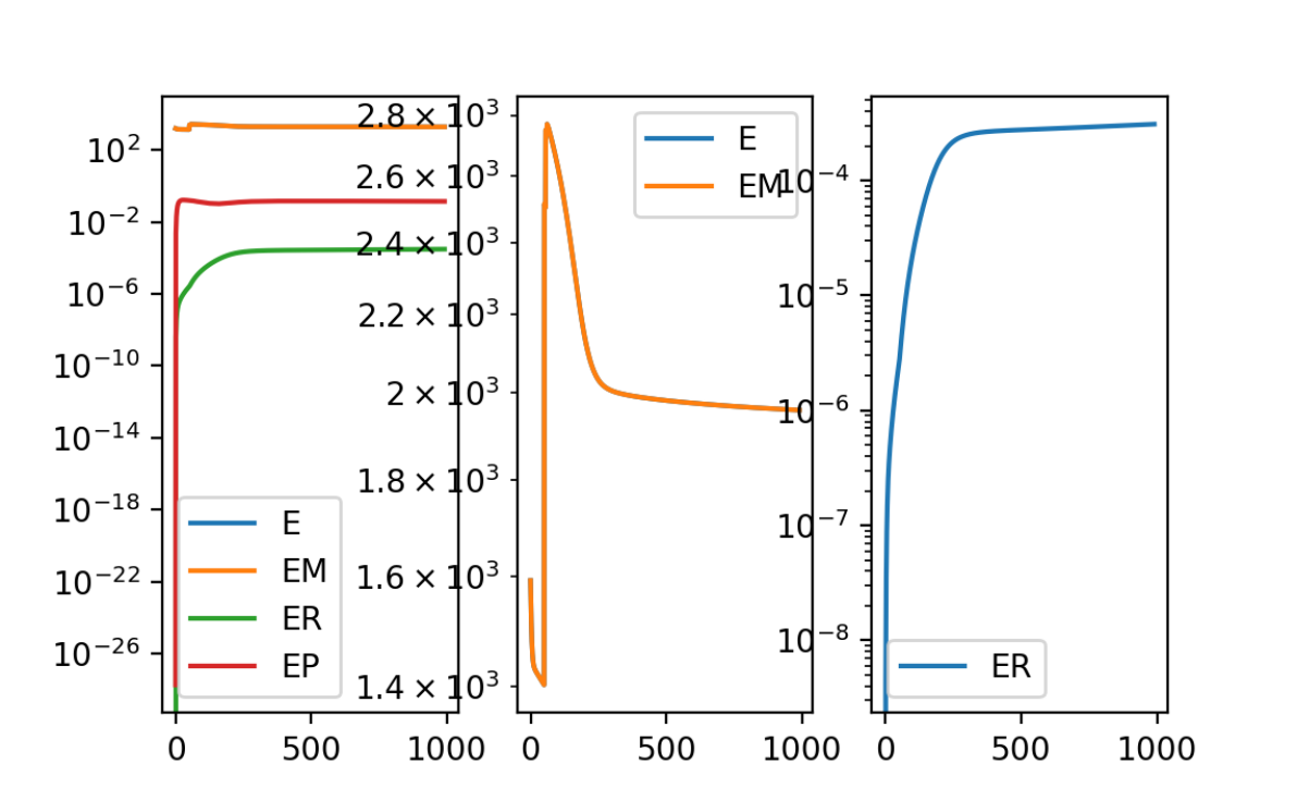
Although we are running with all the same parameters as previously, now the regularization term ER and matching term EM are both plateauing and no longer fluctuating.

## get necessary output variables
A = out['A']
v = out['v']
xv = out['xv']

Again, we can apply the learned transformation to phi to the original non-blurred source image and visualize the results.

# build transformation
phii = STalign.build_transform(xv,v,A,XJ=[YJ,XJ],direction='b')
# apply transformation to Iorig
Iorig = STalign.normalize(V)
Iorig = Iorig.transpose(2,0,1) # convert to [3, 223, 223] tensor 
phiI = STalign.transform_image_source_to_target(xv,v,A,[YI,XI],Iorig,[YJ,XJ])
phiI = phiI.permute(1,2,0).numpy() # convert to [223, 223, 3] numpy matrix for plotting

# plot
fig,ax = plt.subplots(1,3)
ax[0].imshow(phiI)
ax[1].imshow(Jnorm)
ax[2].imshow(phiI)
ax[2].imshow(Jnorm, alpha=0.5)
ax[0].set_title('source with \n LDDMM transform \nusing gaussian blur', fontsize=15)
ax[1].set_title('target', fontsize=15)
ax[2].set_title('combined', fontsize=15)
plt.show()

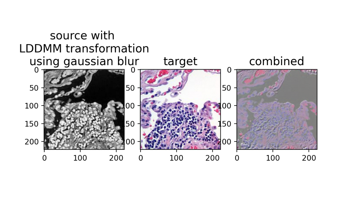
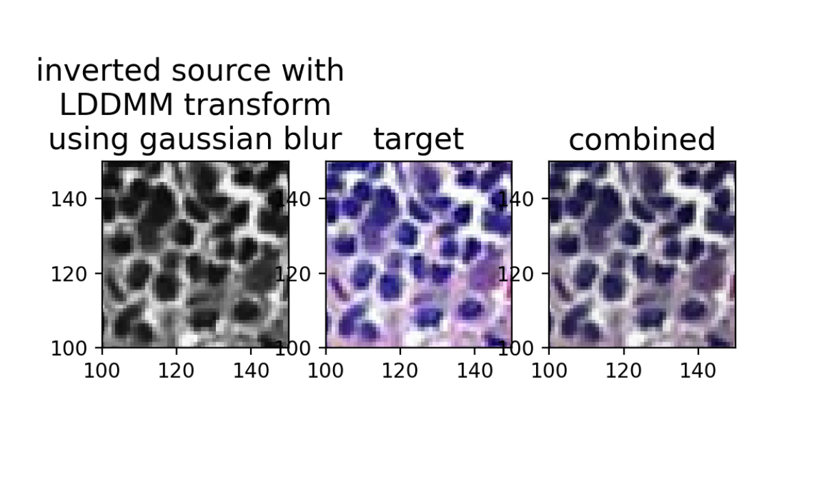
And we have a perfect alignment! To emphasize the single-cell resolution correspondence, we can zoom in and invert the source colors by taking 1 - phiI to visually better match with the target.

# plot
fig,ax = plt.subplots(1,3)
ax[0].imshow(1 - phiI)
ax[1].imshow(Jnorm)
ax[2].imshow(1 - phiI)
ax[2].imshow(Jnorm, alpha=0.5)
ax[0].set_title('inverted source with \n LDDMM transform \nusing gaussian blur', fontsize=15)
ax[1].set_title('target', fontsize=15)
ax[2].set_title('combined', fontsize=15)
ax[0].axis([100,150,100,150])
ax[1].axis([100,150,100,150])
ax[2].axis([100,150,100,150])
plt.show()

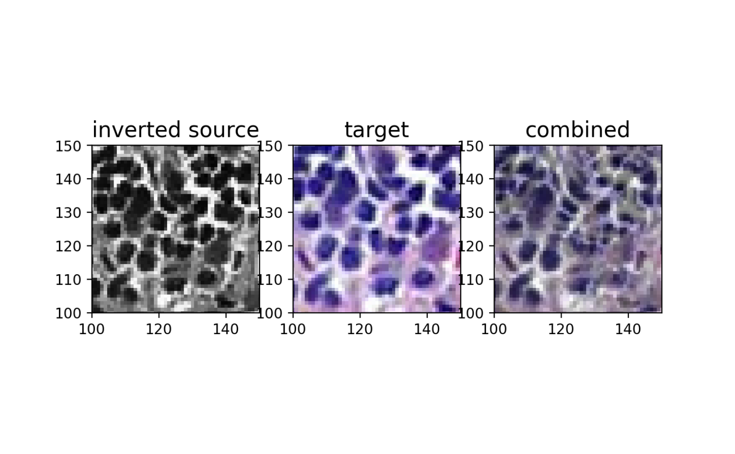
And we can compare with the original source and target image overlay (pre-alignment).

# plot
fig,ax = plt.subplots(1,3)
ax[0].imshow(1 - Inorm)
ax[1].imshow(Jnorm)
ax[2].imshow(1 - Inorm)
ax[2].imshow(Jnorm, alpha=0.5)
ax[0].set_title('inverted source', fontsize=15)
ax[1].set_title('target', fontsize=15)
ax[2].set_title('combined', fontsize=15)
ax[0].axis([100,150,100,150])
ax[1].axis([100,150,100,150])
ax[2].axis([100,150,100,150])
plt.show()

Conclusion

Although in our original publication, we did not demonstrate how STalign could be used to align images from the same tissue at single-cell resolution, by understanding the mathematical underpinnings, we were able to successfully apply STalign to align simulated partially-matched fluorescence and H&E images from the same tissue section at single-cell resolution. I anticipate that real fluorescence and H&E images from the same tissue section will present many more challenges but this demonstration using simulated data is a first step to suggest that such alignment could be feasible using the same underlying mathematical framework!

Try it out for yourself

• Download the images, rotate an image, and see if you can still align them.
• Try placing more/better manual landmarks.
• Change hyperparameters and see what happens.
• Choose a different standard deviation for the Gaussian blur when creating a smooth image representation.