Aligning single-cell resolution spatial transcriptomics data to H&E staining image from Visium

In this notebook, we take a single cell resolution spatial transcriptomics datasets of a coronal section of the adult mouse brain profiled by the MERFISH technology and align it to a H&E staining image from a different individual at matched locations with respect to bregma.

We will use STalign to achieve this alignment. We will first load the relevant code libraries.

## import dependencies
import numpy as np
import matplotlib.pyplot as plt
import matplotlib.transforms as mtransforms
import pandas as pd
import torch
import plotly
import requests

# make plots bigger
plt.rcParams["figure.figsize"] = (12,10)

# OPTION A: import STalign after pip or pipenv install
from STalign import STalign

## OPTION B: skip cell if installed STalign with pip or pipenv
import sys
sys.path.append("../../STalign")

## import STalign from upper directory
import STalign

We can read in the single cell information using pandas as pd.

# Single cell data 1
# read in data
fname = '../merfish_data/datasets_mouse_brain_map_BrainReceptorShowcase_Slice2_Replicate3_cell_metadata_S2R3.csv.gz'
df1 = pd.read_csv(fname)
print(df1.head())

                                Unnamed: 0  fov       volume    center_x
0  158338042824236264719696604356349910479   33   532.778772  617.916619  \
1  260594727341160372355976405428092853003   33  1004.430016  596.808018
2  307643940700812339199503248604719950662   33  1267.183208  578.880018
3   30863303465976316429997331474071348973   33  1403.401822  572.616017
4  313162718584097621688679244357302162401   33   507.949497  608.364018

      center_y       min_x       max_x        min_y        max_y
0  2666.520010  614.725219  621.108019  2657.545209  2675.494810
1  2763.450012  589.669218  603.946818  2757.013212  2769.886812
2  2748.978012  570.877217  586.882818  2740.489211  2757.466812
3  2766.690012  564.937217  580.294818  2756.581212  2776.798812
4  2687.418010  603.061218  613.666818  2682.493210  2692.342810

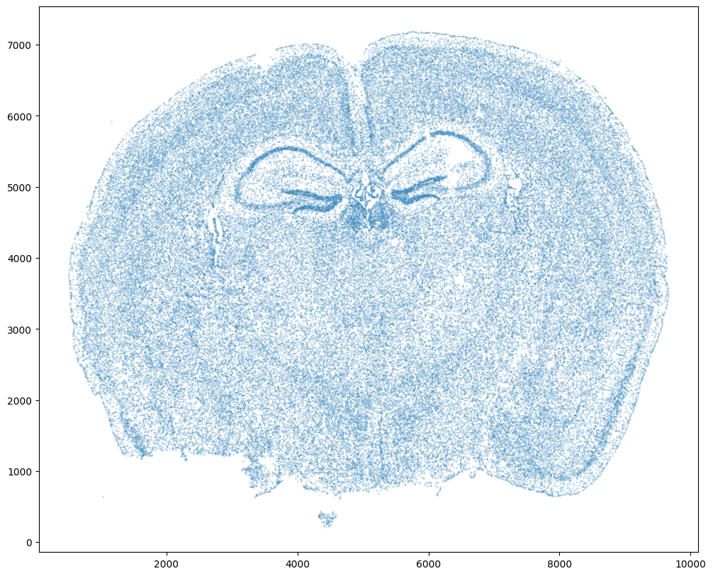
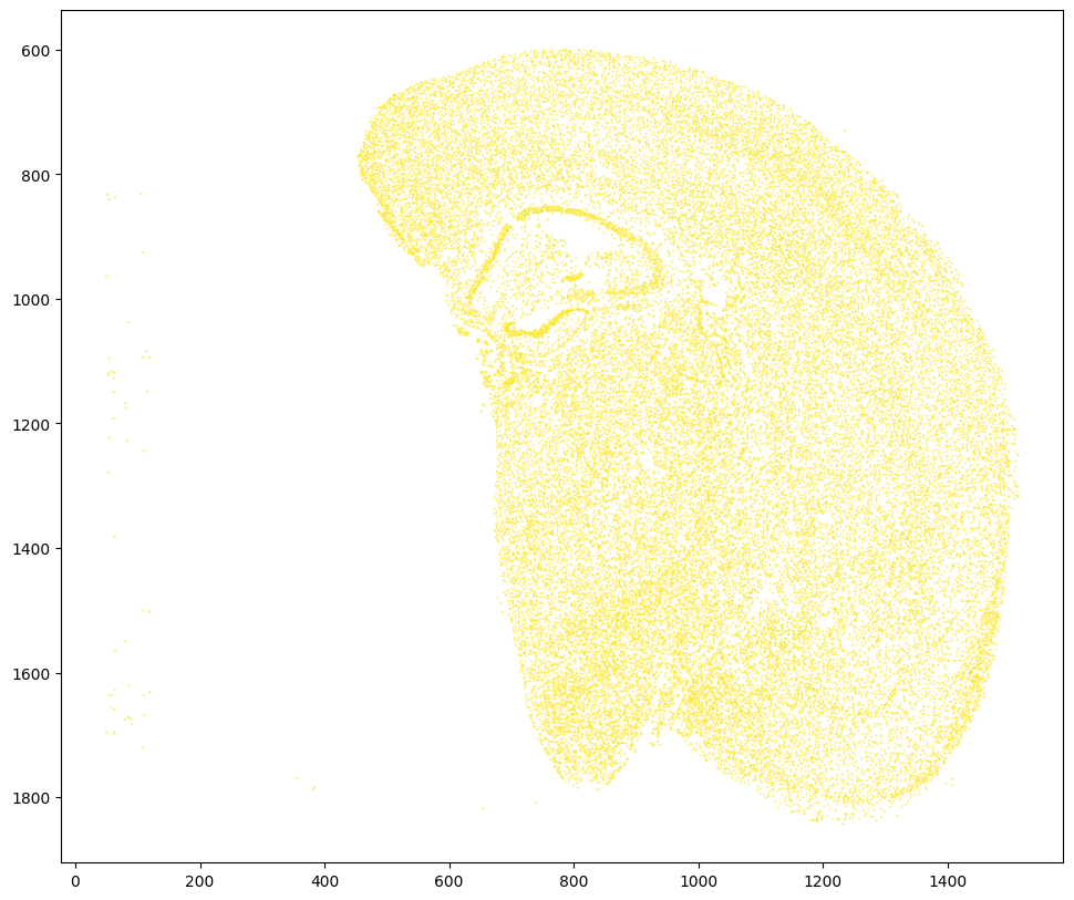
For alignment with STalign, we only need the cell centroid information. So we can pull out this information. We can further visualize the cell centroids to get a sense of the variation in cell density that we will be relying on for our alignment by plotting using matplotlib.pyplot as plt.

# get cell centroid coordinates
xI = np.array(df1['center_x'])
yI = np.array(df1['center_y'])

# plot
fig,ax = plt.subplots()
ax.scatter(xI,yI,s=1,alpha=0.2)
#ax.set_aspect('equal', 'box')

<matplotlib.collections.PathCollection at 0x150872380>

We will use STalign to rasterize the single cell centroid positions into an image. Assuming the single-cell centroid coordinates are in microns, we will perform this rasterization at a 30 micron resolution. We can visualize the resulting rasterized image.

Note that points are plotting with the origin at bottom left while images are typically plotted with origin at top left so we’ve used invert_yaxis() to invert the yaxis for visualization consistency.

# rasterize at 30um resolution (assuming positions are in um units) and plot
XI,YI,I,fig = STalign.rasterize(xI, yI, dx=30)

ax = fig.axes[0]
ax.invert_yaxis()

0 of 85958
10000 of 85958
20000 of 85958
30000 of 85958
40000 of 85958
50000 of 85958
60000 of 85958
70000 of 85958
80000 of 85958
85957 of 85958

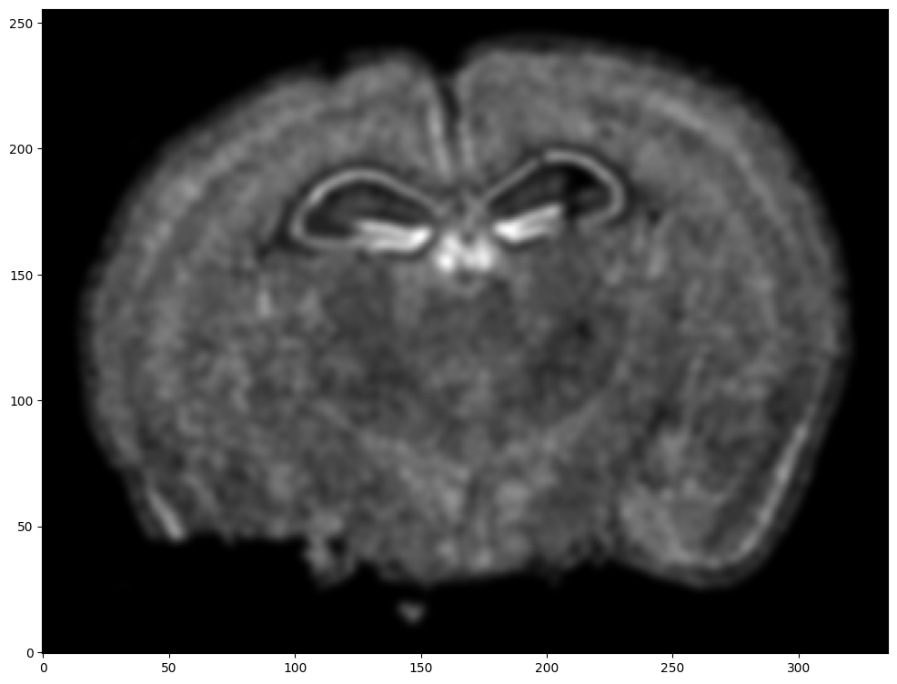
Note that this is a 1D greyscale image. To align with an RGB H&E image, we will need to make our greyscale image into RGB by simply stacking the 1D values 3 times. We will also normalize to get intensity values between 0 to 1.

print("The initial shape of I is {}".format(I.shape))
I = np.vstack((I, I, I)) # make into 3xNxM
print("The range of I is {} to {}".format(I.min(), I.max() ))

# normalize
I = STalign.normalize(I)
print("The range of I after normalization is {} to {}".format(I.min(), I.max() ))

# double check size of things
print("The new shape of I is {}".format(I.shape))

The initial shape of I is (1, 256, 336)
The range of I is 0.0 to 4.715485184477206
The range of I after normalization is 0.0 to 1.0
The new shape of I is (3, 256, 336)

We have already downloaded the H&E staining image from https://www.10xgenomics.com/resources/datasets/adult-mouse-brain-ffpe-1-standard-1-3-0 and placed the file in a folder called visium_data

We can read in the H&E staining image using matplotlib.pyplot as plt.

image_file = '../visium_data/tissue_hires_image.png'
V = plt.imread(image_file)

# plot
fig,ax = plt.subplots()
ax.imshow(V)

<matplotlib.image.AxesImage at 0x152520730>

Note that this is an RGB image that matplotlib.pyplot had read in as an NxMx3 matrix with values ranging from 0 to 1. We will use STalign to normalize the image in case there are any outlier intensities.

print("The initial shape of V is {}".format(V.shape))
print("The range of V is {} to {}".format(V.min(), V.max() ))

Vnorm = STalign.normalize(V)
print("The range of V after normalization is {} to {}".format(Vnorm.min(), Vnorm.max() ))

The initial shape of V is (2000, 1838, 3)
The range of V is 0.10588235408067703 to 1.0
The range of V after normalization is 0.0 to 1.0

We will transpose Vnorm to be a 3xNxM matrix J for downstream analyses. We will also create some variances YJ and XJ to keep track of the image size.

J = Vnorm.transpose(2,0,1)
print("The new shape of J is {}".format(J.shape))

YJ = np.array(range(J.shape[1]))*1. # needs to be longs not doubles for STalign.transform later so multiply by 1.
XJ = np.array(range(J.shape[2]))*1. # needs to be longs not doubles for STalign.transform later so multiply by 1.

The new shape of J is (3, 2000, 1838)

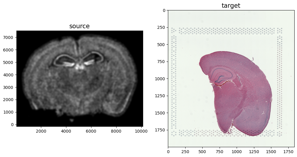
We now have a rasterized image corresponding to the single cell positions from the spatial transcriptomics data and an H&E image that we can align. Note, that we have specified the image from cell positions as source I and the H&E image as target J because the H&E image is only one hemisphere of the brain. We advise choosing the more complete tissue section as the source such that every observation in the target has some correspondence in the source.

# plot

# get extent of images
extentJ = STalign.extent_from_x((YJ,XJ))
extentI = STalign.extent_from_x((YI,XI))

fig,ax = plt.subplots(1,2)
ax[0].imshow((I.transpose(1,2,0).squeeze()), extent=extentI)
ax[0].invert_yaxis()
ax[0].set_title('source', fontsize=15)
ax[1].imshow((J.transpose(1,2,0).squeeze()), extent=extentJ)
ax[1].set_title('target', fontsize=15)

Text(0.5, 1.0, 'target')

Because we desire a partial matching, we incorporated manually placed landmarks to initialize the alignment and further help steer our gradient descent towards an appropriate solution. A point_annotator.py script is provided to assist with this. In order to use the point_annotator.py script, we will need to write out our images as .npz files.

np.savez('../visium_data/Merfish_S2_R3', x=XI,y=YI,I=I)
np.savez('../visium_data/tissue_hires_image', x=XJ,y=YJ,I=J)

Given these .npz files, we can then run the following code on the command line from inside the notebooks folder:

python ../../STalign/point_annotator.py ../visium_data/Merfish_S2_R3.npz ../visium_data/tissue_hires_image.npz

Which will provide a graphical user interface (GUI) to selecting points. Once you run the code, the command line will prompt you to enter the name of a landmark point. Then, you will be prompted on the GUI to select and save the landmark point for both source and target images. You can annotate multiple landmark points with the same name, and each of them would have an index at the end (e.g. “CA0” and “CA1” in this tutorial). However, when doing so, make sure to annotate landmark points alternatively on source and target to avoid any error. You can annotate multiple landmark points with different names by repeating the process of entering the name for a landmark point, following the GUI prompts, and returning to the command line to enter the name for the next landmark point.

Annotated points will saved as Merfish_S2_R3_points.npy and tissue_hires_image_points.npy respectively. We can then read in these files.

# read from file
pointsIlist = np.load('../visium_data/Merfish_S2_R3_points.npy', allow_pickle=True).tolist()
print(pointsIlist)
pointsJlist = np.load('../visium_data/tissue_hires_image_points.npy', allow_pickle=True).tolist()
print(pointsJlist)

{'RSP': [(5095.02260152, 5499.7972588), (4910.8223317, 6628.02391148), (5463.42314117, 7019.44948485)], 'DG-sg': [(5532.49824236, 4901.14638187), (6131.14911929, 4832.07128069), (6223.2492542, 5131.39671915)], 'CA': [(5371.32300626, 5269.54692152), (6154.17415302, 5753.07262981), (6683.74992876, 5591.89739371), (6937.02529977, 5246.52188779)], 'PAA': [(8111.3020199, 641.51514218)], 'MEAav': [(6937.02529977, 963.86561437)]}
{'RSP': [(559.82404846, 938.72950082), (463.88640793, 788.82693749), (505.85912566, 674.90098936)], 'DG-sg': [(709.72661179, 1046.65934642), (823.65255993, 1022.67493629), (799.66814979, 956.71780842)], 'CA': [(631.77727886, 1016.67883376), (733.71102193, 860.78016789), (859.62917513, 878.76847549), (949.57071313, 962.71391096)], 'PAA': [(1267.3641474, 1826.15267576)], 'MEAav': [(955.56681566, 1694.23842003)]}

Note that these landmark points are read in as lists. We will want to convert them to a simple array for downstream usage.

# convert to array
pointsI = []
pointsJ = []

for i in pointsIlist.keys():
    for j in range(len(pointsIlist[i])):
        pointsI.append([pointsIlist[i][j][1], pointsIlist[i][j][0]])
for i in pointsJlist.keys():
    for j in range(len(pointsJlist[i])):
        pointsJ.append([pointsJlist[i][j][1], pointsJlist[i][j][0]])

pointsI = np.array(pointsI)
pointsJ = np.array(pointsJ)

# now arrays
print(pointsI)
print(pointsJ)

[[5499.7972588  5095.02260152]
 [6628.02391148 4910.8223317 ]
 [7019.44948485 5463.42314117]
 [4901.14638187 5532.49824236]
 [4832.07128069 6131.14911929]
 [5131.39671915 6223.2492542 ]
 [5269.54692152 5371.32300626]
 [5753.07262981 6154.17415302]
 [5591.89739371 6683.74992876]
 [5246.52188779 6937.02529977]
 [ 641.51514218 8111.3020199 ]
 [ 963.86561437 6937.02529977]]
[[ 938.72950082  559.82404846]
 [ 788.82693749  463.88640793]
 [ 674.90098936  505.85912566]
 [1046.65934642  709.72661179]
 [1022.67493629  823.65255993]
 [ 956.71780842  799.66814979]
 [1016.67883376  631.77727886]
 [ 860.78016789  733.71102193]
 [ 878.76847549  859.62917513]
 [ 962.71391096  949.57071313]
 [1826.15267576 1267.3641474 ]
 [1694.23842003  955.56681566]]

We can double check that our landmark points look sensible by plotting them along with the rasterized image we created.

# plot

fig,ax = plt.subplots(1,2)
ax[0].imshow((I.transpose(1,2,0).squeeze()), extent=extentI)
ax[1].imshow((J.transpose(1,2,0).squeeze()), extent=extentJ)

trans_offset_0 = mtransforms.offset_copy(ax[0].transData, fig=fig,
                                       x=0.05, y=-0.05, units='inches')
trans_offset_1 = mtransforms.offset_copy(ax[1].transData, fig=fig,
                                       x=0.05, y=-0.05, units='inches')

ax[0].scatter(pointsI[:,1],pointsI[:,0], c='red', s=10)
ax[1].scatter(pointsJ[:,1],pointsJ[:,0], c='red', s=10)

for i in pointsIlist.keys():
    for j in range(len(pointsIlist[i])):
        ax[0].text(pointsIlist[i][j][0], pointsIlist[i][j][1],f'{i}{j}', c='red', transform=trans_offset_0, fontsize= 8)
for i in pointsJlist.keys():
    for j in range(len(pointsJlist[i])):
        ax[1].text(pointsJlist[i][j][0], pointsJlist[i][j][1],f'{i}{j}', c='red', transform=trans_offset_1, fontsize= 8)

ax[0].set_title('source with pointsI', fontsize=15)
ax[1].set_title('target with pointsJ', fontsize=15)

# invert only rasterized image
ax[0].invert_yaxis()

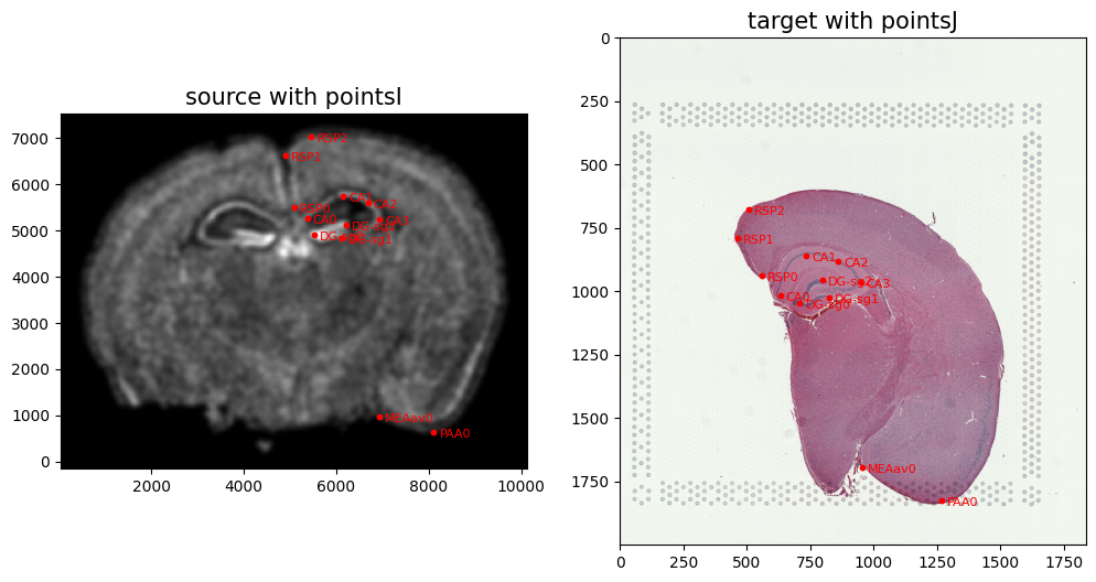
From the landmark points, we can generate a linear transformation L and translation T which will produce a simple initial affine transformation A.

# set device for building tensors
if torch.cuda.is_available():
    torch.set_default_device('cuda:0')
else:
    torch.set_default_device('cpu')

# compute initial affine transformation from points
L,T = STalign.L_T_from_points(pointsI,pointsJ)
A = STalign.to_A(torch.tensor(L),torch.tensor(T))

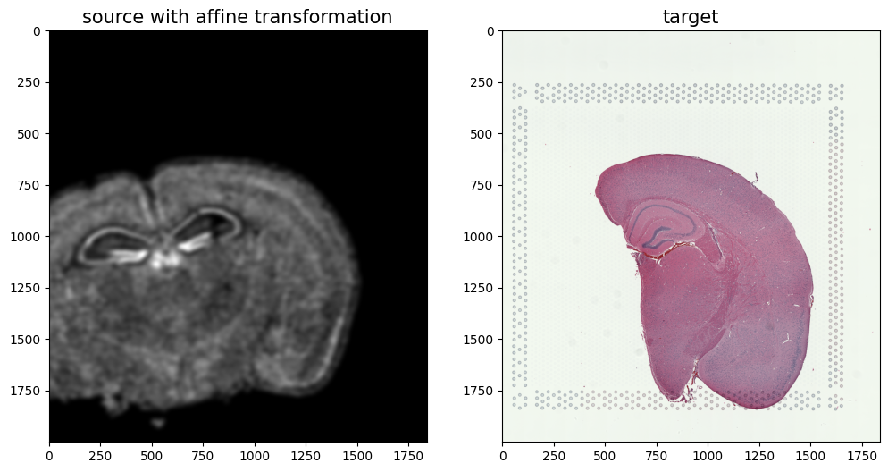
We can show the results of the simple affine transformation.

# compute initial affine transformation from points
AI= STalign.transform_image_source_with_A(A, [YI,XI], I, [YJ,XJ])

#switch tensor from cuda to cpu for plotting with numpy
if AI.is_cuda:
    AI = AI.cpu()

fig,ax = plt.subplots(1,2)

ax[0].imshow((AI.permute(1,2,0).squeeze()), extent=extentJ)
ax[1].imshow((J.transpose(1,2,0).squeeze()), extent=extentJ)

ax[0].set_title('source with affine transformation', fontsize=15)
ax[1].set_title('target', fontsize=15)

/Users/kalenclifton/.local/share/virtualenvs/STalign-wXTCUYXW/lib/python3.10/site-packages/torch/utils/_device.py:62: UserWarning: To copy construct from a tensor, it is recommended to use sourceTensor.clone().detach() or sourceTensor.clone().detach().requires_grad_(True), rather than torch.tensor(sourceTensor).
  return func(*args, **kwargs)

Text(0.5, 1.0, 'target')

#apply A to sources points in row, column (y,x) orientation
affine = np.matmul(np.array(A.cpu()),np.array([yI, xI, np.ones(len(xI))]))

xIaffine = affine[1,:]
yIaffine = affine[0,:]


#apply A to sources landmark points in row, column (y,x) orientation
ypointsI = pointsI[:,0]
xpointsI = pointsI[:,1]
affine = np.matmul(np.array(A.cpu()),np.array([ypointsI, xpointsI, np.ones(len(ypointsI))]))

xpointsIaffine = affine[1,:]
ypointsIaffine = affine[0,:]
pointsIaffine = np.column_stack((ypointsIaffine,xpointsIaffine))


# plot results
fig,ax = plt.subplots()

ax.imshow((J).transpose(1,2,0),extent=extentJ)

ax.scatter(xIaffine,yIaffine,s=1,alpha=0.1, label = 'source aligned')
ax.scatter(pointsIaffine[:,1],pointsIaffine[:,0],c="blue", label='source landmarks aligned', s=100)

ax.scatter(pointsJ[:,1],pointsJ[:,0], c='red', label='target landmarks', s=100)
ax.set_aspect('equal')

lgnd = plt.legend(loc="upper right", scatterpoints=1, fontsize=10)
for handle in lgnd.legend_handles:
    handle.set_sizes([10.0])

ax.set_title('Landmark-based Affine Alignment', fontsize=15)

Text(0.5, 1.0, 'Landmark-based Affine Alignment')

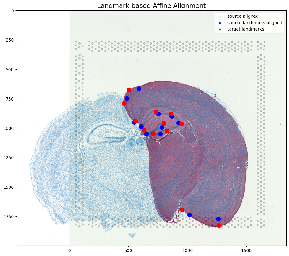
In this case, we can observe that a simple affine alignment is not sufficient to align the single-cell spatial transcriptomics dataset to the H&E staining image. So we will need to perform non-linear local alignments via LDDMM.

%%time

# run LDDMM
# specify device (default device for STalign.LDDMM is cpu)
if torch.cuda.is_available():
    device = 'cuda:0'
else:
    device = 'cpu'

# keep all other parameters default
params = {'L':L,'T':T,
          'niter': 200,
          'pointsI': pointsI,
          'pointsJ': pointsJ,
          'device': device,
          'sigmaP': 2e-1,
          'sigmaM': 0.18,
          'sigmaB': 0.18,
          'sigmaA': 0.18,
          'diffeo_start' : 100,
          'epL': 5e-11,
          'epT': 5e-4,
          'epV': 5e1
          }

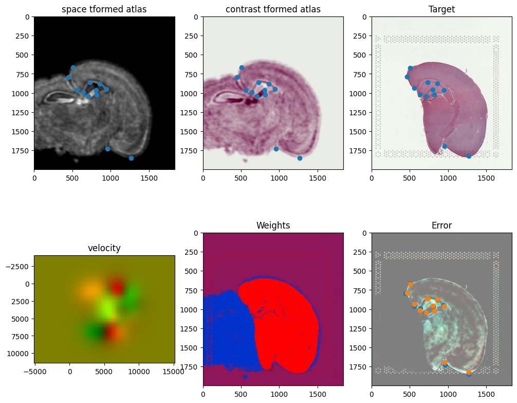
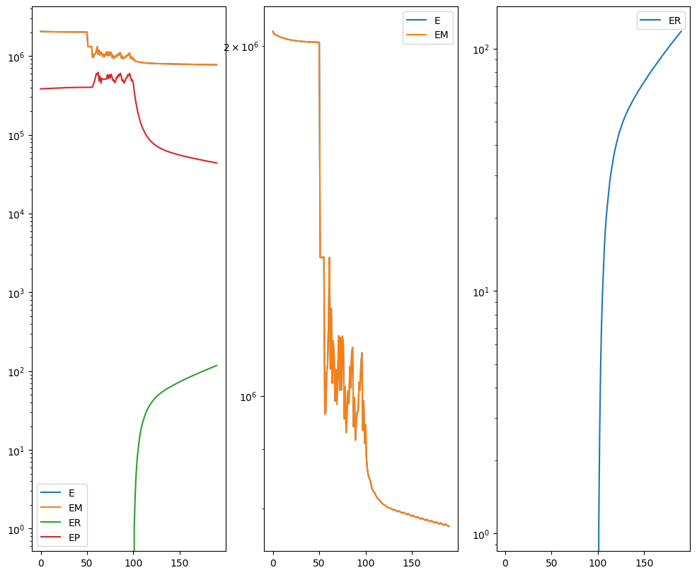
out = STalign.LDDMM([YI,XI],I,[YJ,XJ],J,**params)

/home/kalen/.local/share/virtualenvs/STalign-VWNsoi3D/lib/python3.8/site-packages/torch/functional.py:504: UserWarning: torch.meshgrid: in an upcoming release, it will be required to pass the indexing argument. (Triggered internally at ../aten/src/ATen/native/TensorShape.cpp:3483.)
  return _VF.meshgrid(tensors, **kwargs)  # type: ignore[attr-defined]
/home/kalen/STalign/docs/notebooks/../../STalign/STalign.py:1301: UserWarning: Data has no positive values, and therefore cannot be log-scaled.
  axE[2].set_yscale('log')
/home/kalen/.local/share/virtualenvs/STalign-VWNsoi3D/lib/python3.8/site-packages/matplotlib/cm.py:478: RuntimeWarning: invalid value encountered in cast
  xx = (xx * 255).astype(np.uint8)

CPU times: user 5min 26s, sys: 29.5 s, total: 5min 55s
Wall time: 5min 28s

#### get necessary output variables
A = out['A']
v = out['v']
xv = out['xv']
WM = out['WM']

Plots generated throughout the alignment can be used to give you a sense of whether the parameter choices are appropriate and whether your alignment is converging on a solution.

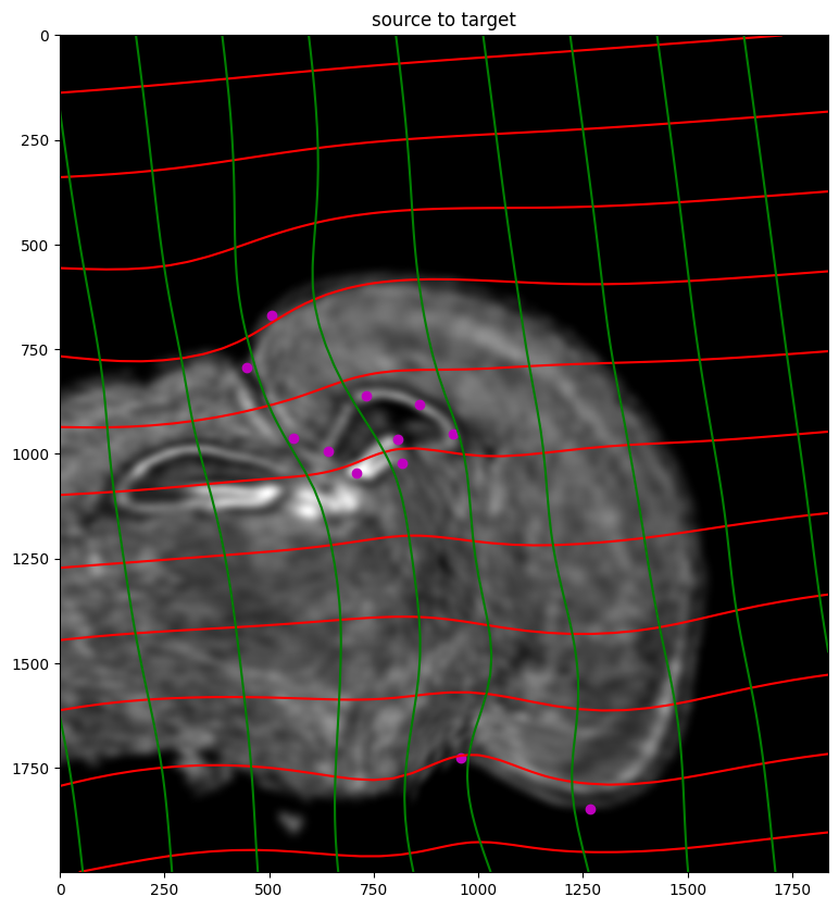
We can also evaluate the resulting alignment by applying the transformation to visualize how our source and target images were deformed to achieve the alignment.

# apply transform
phii = STalign.build_transform(xv,v,A,XJ=[YJ,XJ],direction='b')
phiI = STalign.transform_image_source_to_target(xv,v,A,[YI,XI],I,[YJ,XJ])
phiipointsI = STalign.transform_points_source_to_target(xv,v,A,pointsI)

#switch tensor from cuda to cpu for plotting with numpy
if phii.is_cuda:
    phii = phii.cpu()
if phiI.is_cuda:
    phiI = phiI.cpu()
if phiipointsI.is_cuda:
    phiipointsI = phiipointsI.cpu()


# plot with grids
fig,ax = plt.subplots()
levels = np.arange(-100000,100000,1000)

ax.contour(XJ,YJ,phii[...,0],colors='r',linestyles='-',levels=levels)
ax.contour(XJ,YJ,phii[...,1],colors='g',linestyles='-',levels=levels)
ax.set_aspect('equal')
ax.set_title('source to target')

ax.imshow(phiI.permute(1,2,0)/torch.max(phiI),extent=extentJ)
ax.scatter(phiipointsI[:,1].detach(),phiipointsI[:,0].detach(),c="m")

<matplotlib.collections.PathCollection at 0x7fb0605682b0>

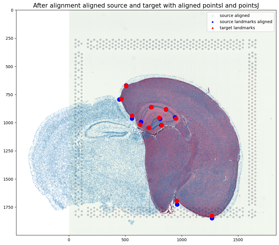
Finally, we can apply our transform to the original sets of single cell centroid positions to achieve their new aligned positions.

# apply transform to original points
tpointsI= STalign.transform_points_source_to_target(xv,v,A, np.stack([yI, xI], 1))

#switch tensor from cuda to cpu for plotting with numpy
if tpointsI.is_cuda:
    tpointsI = tpointsI.cpu()

# switch from row column coordinates (y,x) to (x,y)
xI_LDDMM = tpointsI[:,1]
yI_LDDMM = tpointsI[:,0]

And we can visualize the results.

# plot results
fig,ax = plt.subplots()

ax.imshow((J).transpose(1,2,0),extent=extentJ)

ax.scatter(xI_LDDMM,yI_LDDMM,s=1,alpha=0.1, label = 'source aligned')
ax.scatter(phiipointsI[:,1].detach(),phiipointsI[:,0].detach(),c="blue", label='source landmarks aligned', s=100)

ax.scatter(pointsJ[:,1],pointsJ[:,0], c='red', label='target landmarks', s=100)
ax.set_aspect('equal')

lgnd = plt.legend(loc="upper right", scatterpoints=1, fontsize=10)
for handle in lgnd.legend_handles:
    handle.set_sizes([10.0])

ax.set_title('After alignment aligned source and target with aligned pointsI and pointsJ', fontsize=15)

Text(0.5, 1.0, 'After alignment aligned source and target with aligned pointsI and pointsJ')

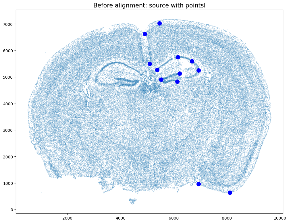
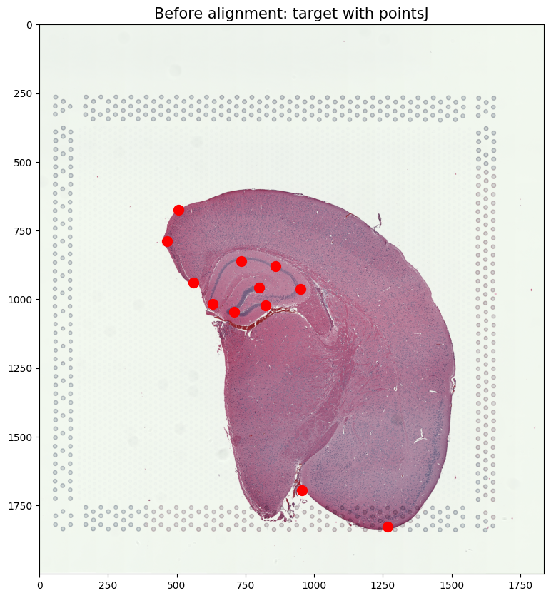
Reminder of what source and target looked like before alignment

# plot
fig,ax = plt.subplots()
ax.scatter(xI,yI,s=1,alpha=0.2)
ax.set_aspect('equal', 'box')
ax.scatter(pointsI[:,1],pointsI[:,0], c='blue', s=100)
ax.set_title('Before alignment: source with pointsI', fontsize=15)

Text(0.5, 1.0, 'Before alignment: source with pointsI')

fig,ax = plt.subplots()
ax.imshow((J.transpose(1,2,0).squeeze()), extent=extentJ)
ax.scatter(pointsJ[:,1],pointsJ[:,0], c='red', s=100)
ax.set_title('Before alignment: target with pointsJ', fontsize=15)

Text(0.5, 1.0, 'Before alignment: target with pointsJ')

Save the new aligned positions by appending to our original data

if tpointsI.is_cuda:
    df3 = pd.DataFrame(

        {

            "aligned_x": xI_LDDMM.cpu(),

            "aligned_y": yI_LDDMM.cpu(),

        },


    )
else:
    df3 = pd.DataFrame(

        {

            "aligned_x": xI_LDDMM,

            "aligned_y": yI_LDDMM,

        },


    )
results = pd.concat([df1, df3], axis=1)
results.head()

	Unnamed: 0	fov	volume	center_x	center_y	min_x	max_x	min_y	max_y	aligned_x	aligned_y
0	158338042824236264719696604356349910479	33	532.778772	617.916619	2666.520010	614.725219	621.108019	2657.545209	2675.494810	-304.781922	1543.947789
1	260594727341160372355976405428092853003	33	1004.430016	596.808018	2763.450012	589.669218	603.946818	2757.013212	2769.886812	-311.687871	1526.968682
2	307643940700812339199503248604719950662	33	1267.183208	578.880018	2748.978012	570.877217	586.882818	2740.489211	2757.466812	-314.931483	1530.063358
3	30863303465976316429997331474071348973	33	1403.401822	572.616017	2766.690012	564.937217	580.294818	2756.581212	2776.798812	-316.678395	1527.017231
4	313162718584097621688679244357302162401	33	507.949497	608.364018	2687.418010	603.061218	613.666818	2682.493210	2692.342810	-307.285999	1540.425385

We will finally create a compressed .csv.gz file named mouse_brain_map_BrainReceptorShowcase_Slice2_Replicate3_STalign_to_Visium_tissue_hires_image_with_point_annotator.csv.gz

results.to_csv('../merfish_data/mouse_brain_map_BrainReceptorShowcase_Slice2_Replicate3_STalign_to_Visium_tissue_hires_image_with_point_annotator.csv.gz',
               compression='gzip')

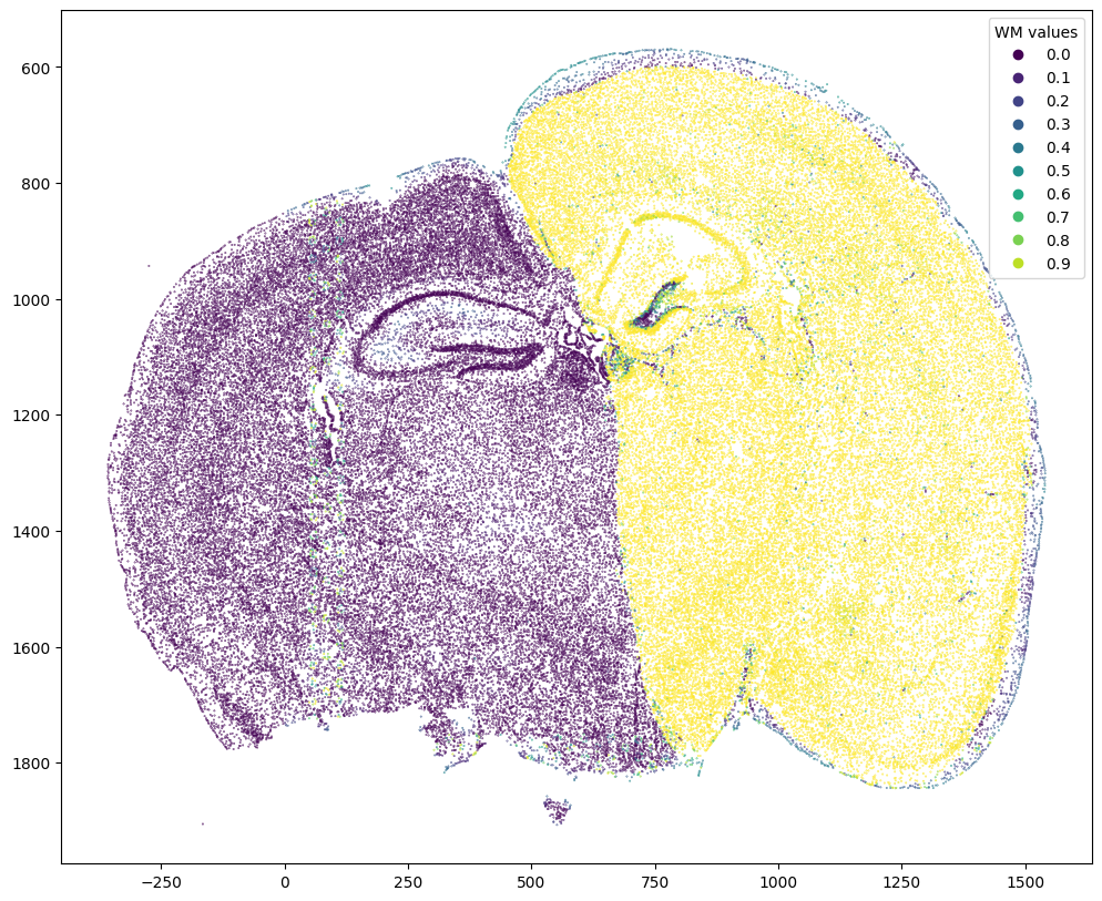
We can also remove background cells in the MERFISH data that did not have a target H&E staining image. Here, we compute weight values for transformed source MERFISH points from target H&E image pixel locations and weight 2D array (matching). We then use the computed weight values and a manually selected threshold to remove background cells.

# compute weight values for transformed source points from target image pixel locations and weight 2D array (matching)
testM = STalign.interp([YJ,XJ],WM[None].float(),tpointsI[None].permute(-1,0,1).float())

#switch tensor from cuda to cpu for plotting with numpy
if testM.is_cuda:
    testM = testM.cpu()

fig,ax = plt.subplots()
scatter = ax.scatter(tpointsI[:,1],tpointsI[:,0],c=testM[0,0],s=0.1,vmin=0,vmax=1, label='WM values')
legend1 = ax.legend(*scatter.legend_elements(),
                    loc="upper right", title="WM values")
ax.invert_yaxis()

# save weight values
results['WM_values'] = testM[0,0]

results

	Unnamed: 0	fov	volume	center_x	center_y	min_x	max_x	min_y	max_y	aligned_x	aligned_y	WM_values
0	158338042824236264719696604356349910479	33	532.778772	617.916619	2666.520010	614.725219	621.108019	2657.545209	2675.494810	-304.781922	1543.947789	0.000000
1	260594727341160372355976405428092853003	33	1004.430016	596.808018	2763.450012	589.669218	603.946818	2757.013212	2769.886812	-311.687871	1526.968682	0.000000
2	307643940700812339199503248604719950662	33	1267.183208	578.880018	2748.978012	570.877217	586.882818	2740.489211	2757.466812	-314.931483	1530.063358	0.000000
3	30863303465976316429997331474071348973	33	1403.401822	572.616017	2766.690012	564.937217	580.294818	2756.581212	2776.798812	-316.678395	1527.017231	0.000000
4	313162718584097621688679244357302162401	33	507.949497	608.364018	2687.418010	603.061218	613.666818	2682.493210	2692.342810	-307.285999	1540.425385	0.000000
...	...	...	...	...	...	...	...	...	...	...	...	...
85953	311704042603434891559886168438769992293	1545	1625.490809	9623.123579	4030.182069	9615.660779	9630.586379	4019.749269	4040.614869	1519.770766	1175.919074	0.387589
85954	312851880059098327776181257829209599759	1545	905.032435	9625.067579	4008.749469	9620.088779	9630.046379	4000.320068	4017.178869	1520.722933	1180.469056	0.349814
85955	332299915869590281339501510603978852698	1545	459.647325	9605.470978	4187.268073	9600.767578	9610.174378	4182.397273	4192.138873	1511.553158	1142.686375	0.398904
85956	150462787759670321084458536479486602685	1546	778.386670	9606.874978	4208.819338	9600.767578	9612.982378	4200.335938	4217.302738	1511.134796	1138.034522	0.374337
85957	268870416870774615427277589169474700725	1546	592.088115	9607.841578	4219.019938	9602.700778	9612.982378	4213.393138	4224.646738	1510.995518	1135.826149	0.364696

85958 rows × 12 columns

fig,ax = plt.subplots()
ax.hist(results['WM_values'], bins = 20)

(array([41242.,   842.,   535.,   439.,   376.,   359.,   358.,   258.,
          204.,   217.,   153.,   129.,   145.,   170.,   194.,   214.,
          293.,   356.,   708., 38766.]),
 array([0.        , 0.0499999 , 0.09999981, 0.14999971, 0.19999962,
        0.24999952, 0.29999942, 0.34999934, 0.39999923, 0.44999915,
        0.49999905, 0.54999894, 0.59999883, 0.64999878, 0.69999868,
        0.74999857, 0.79999846, 0.84999835, 0.89999831, 0.9499982 ,
        0.99999809]),
 <BarContainer object of 20 artists>)

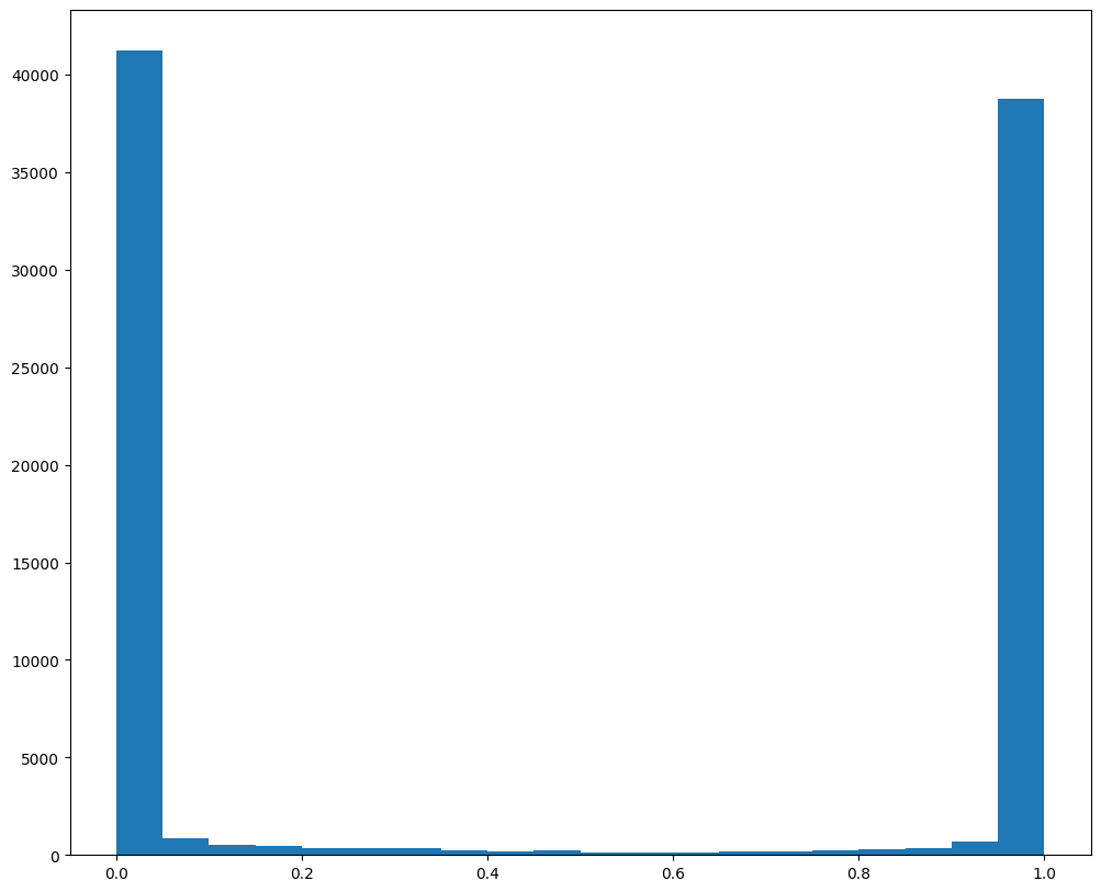
Based on this distribution and manual inspection, we can manually set a threshold value to filter transformed MERFISH data.

# set a threshold value
WMthresh = .95

# filter transformed MERFISH data
results_filtered = results[results['WM_values'] > WMthresh]

# plot
fig,ax = plt.subplots()
ax.scatter(results_filtered['aligned_x'],results_filtered['aligned_y'],c=results_filtered['WM_values'],s=0.1,vmin=0,vmax=1)
ax.set_aspect('equal')
ax.invert_yaxis()
plt.show()

Similar to the unfiltered dataset, create a compressed .csv.gz file named mouse_brain_map_BrainReceptorShowcase_Slice2_Replicate3_STalign_to_Slice2_Replicate2_STalign_to_Visium_tissue_hires_image_with_point_annotator_filtered.csv.gz

results.to_csv('../merfish_data/mouse_brain_map_BrainReceptorShowcase_Slice2_Replicate3_STalign_to_Slice2_Replicate2_STalign_to_Visium_tissue_hires_image_with_point_annotator_filtered.csv.gz',
               compression='gzip')