Aligning single-cell resolution breast cancer spatial transcriptomics data to corresponding H&E staining image from Xenium

In this notebook, we take a single cell resolution spatial transcriptomics datasets of a breast cancer section profiled by the Xenium technology and align it to a corresponding H&E staining image of the same tissue section. See the bioRxiv preprint for more details about this data: https://www.biorxiv.org/content/10.1101/2022.10.06.510405v2

According to the authors, “Due to the non-destructive nature of the Xenium workflow, we were able to perform H&E staining…on the same section post-processing.” However, as the H&E staining and imaging was done seprately to the spatial transcriptomics data collection, alignment is still needed to register the H&E staining image with the single cell positions from the spatial transcriptomics data.

We will use STalign to achieve this alignment. We will first load the relevant code libraries.

# import dependencies
import numpy as np
import matplotlib.pyplot as plt
import pandas as pd
import torch

# make plots bigger
plt.rcParams["figure.figsize"] = (12,10)

# OPTION A: import STalign after pip or pipenv install
from STalign import STalign

## OPTION B: skip cell if installed STalign with pip or pipenv
import sys
sys.path.append("../../STalign")

## import STalign from upper directory
import STalign

To obtain the single cell spatial transcriptomics data, we can download the Xenium Output Bundle from the 10X website: https://www.10xgenomics.com/products/xenium-in-situ/preview-dataset-human-breast Expanding the downloaded Xenium_FFPE_Human_Breast_Cancer_Rep1_outs.zip, we will use the single cell positions stored in cells.csv.gz. Likewise, we can download the accompanying H&E staining image Supplemental: Post-Xenium H&E image (TIFF) as Xenium_FFPE_Human_Breast_Cancer_Rep1_he_image.tif.

To reproduce this tutorial, we have placed these files in a folder called `xenium_data/ <https://github.com/JEFworks-Lab/STalign/tree/main/docs/xenium_data>`__ with cells.csv.gz renamed as Xenium_FFPE_Human_Breast_Cancer_Rep1_cells.csv.gz for organizational purposes. Likewise, to minimize storage, we have resized the high resolution H&E TIF image into a smaller PNG image as Xenium_FFPE_Human_Breast_Cancer_Rep1_he_image.png

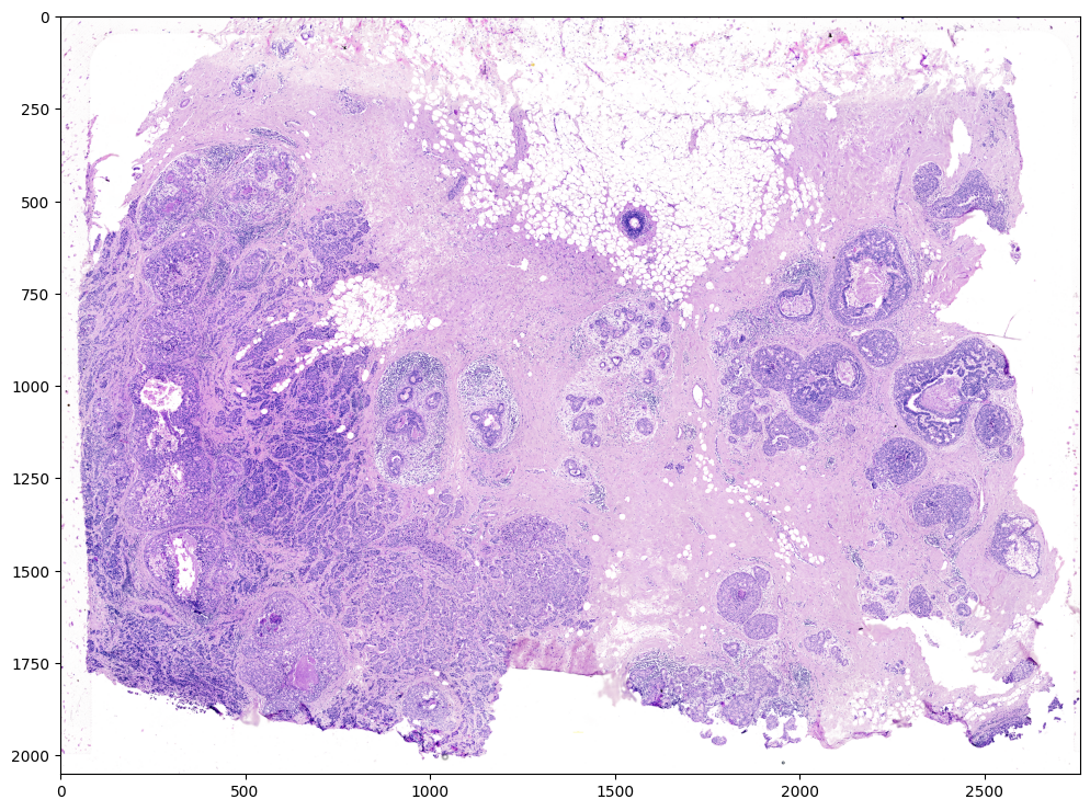
We can read in the H&E staining image using matplotlib.pyplot as plt.

# Target is H&E staining image
image_file = '../xenium_data/Xenium_FFPE_Human_Breast_Cancer_Rep1_he_image.png'
V = plt.imread(image_file)

# plot
fig,ax = plt.subplots()
ax.imshow(V)

<matplotlib.image.AxesImage at 0x17e205e10>

Note that this is an RGB image that matplotlib.pyplot had read in as an NxMx3 matrix with values ranging from 0 to 1.

print(V.shape)
print(V.min())
print(V.max())

(2051, 2759, 3)
0.0
1.0

We will use STalign to normalize the image in case there are any outlier intensities.

Inorm = STalign.normalize(V)

print(Inorm.min())
print(Inorm.max())

fig,ax = plt.subplots()
ax.imshow(Inorm)

0.0
1.0

<matplotlib.image.AxesImage at 0x17e03e3e0>

We will transpose Inorm to be a 3xNxM matrix for downstream analyses. We will also create some variances YI and XI to keep track of the image size.

I = Inorm.transpose(2,0,1)
print(I.shape)

YI = np.array(range(I.shape[1]))*1. # needs to be longs not doubles for STalign.transform later so multiply by 1.
XI = np.array(range(I.shape[2]))*1. # needs to be longs not doubles for STalign.transform later so multiply by 1.
extentI = STalign.extent_from_x((YI,XI))

(3, 2051, 2759)

We can also now read in the corresponding single cell information using pandas as pd.

# Single cell data to be aligned
fname = '../xenium_data/Xenium_FFPE_Human_Breast_Cancer_Rep1_cells.csv.gz'
df = pd.read_csv(fname)
df.head()

	cell_id	x_centroid	y_centroid	transcript_counts	control_probe_counts	control_codeword_counts	total_counts	cell_area	nucleus_area
0	1	377.663005	843.541888	154	0	0	154	110.361875	45.562656
1	2	382.078658	858.944818	64	0	0	64	87.919219	24.248906
2	3	319.839529	869.196542	57	0	0	57	52.561875	23.526406
3	4	259.304707	851.797949	120	0	0	120	75.230312	35.176719
4	5	370.576291	865.193024	120	0	0	120	180.218594	34.499375

For alignment with STalign, we only need the cell centroid information. So we can pull out this information. We can further visualize the cell centroids to get a sense of the variation in cell density that we will be relying on for our alignment by plotting using matplotlib.pyplot as plt.

# get cell centroid coordinates
xM = np.array(df['x_centroid'])
yM = np.array(df['y_centroid'])

# plot
fig,ax = plt.subplots()
ax.scatter(xM,yM,s=1,alpha=0.2)

<matplotlib.collections.PathCollection at 0x17f527ac0>

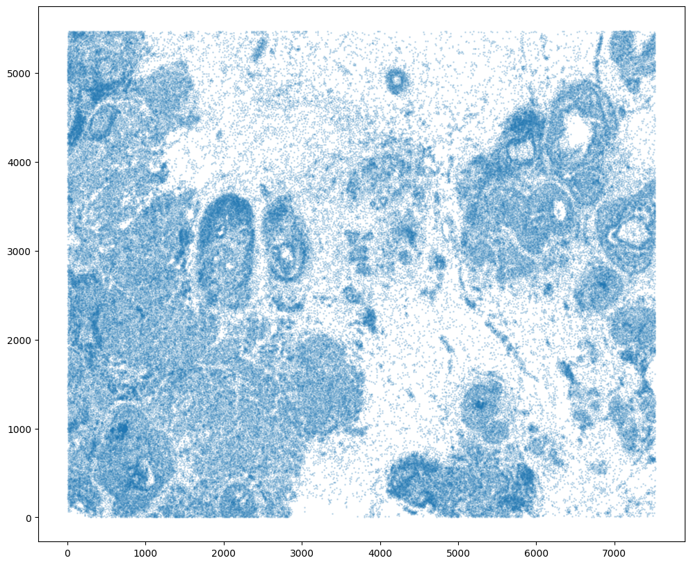
Note that plotting the cell centroid positions on the corresponding H&E image shows that alignment is still needed.

# plot
fig,ax = plt.subplots()
ax.imshow((I).transpose(1,2,0),extent=extentI)
ax.scatter(xM,yM,s=1,alpha=0.1)

<matplotlib.collections.PathCollection at 0x17f3eba00>

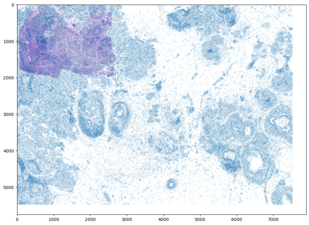
To begin our alignment, we will use STalign to rasterize the single cell centroid positions into an image. Assuming the single-cell centroid coordinates are in microns, we will perform this rasterization at a 30 micron resolution. We can visualize the resulting rasterized image.

Note that points are plotting with the origin at bottom left while images are typically plotted with origin at top left so we’ve used invert_yaxis() to invert the yaxis for visualization consistency.

# rasterize at 30um resolution (assuming positions are in um units) and plot
XJ,YJ,M,fig = STalign.rasterize(xM, yM, dx=30)

ax = fig.axes[0]
ax.invert_yaxis()

0 of 167782
10000 of 167782
20000 of 167782
30000 of 167782
40000 of 167782
50000 of 167782
60000 of 167782
70000 of 167782
80000 of 167782
90000 of 167782
100000 of 167782
110000 of 167782
120000 of 167782
130000 of 167782
140000 of 167782
150000 of 167782
160000 of 167782
167781 of 167782

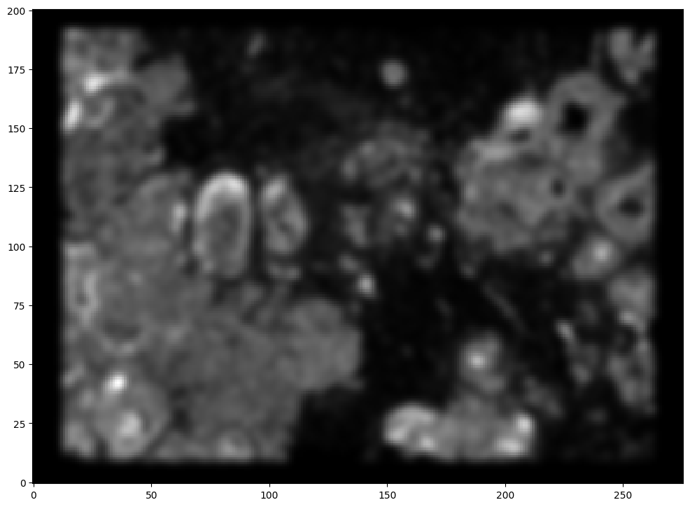
Note that this is a 1D greyscale image. To align with an RGB H&E image, we will need to make our greyscale image into RGB by simply stacking the 1D values 3 times. We will also normalize to get intensity values between 0 to 1. We now have an H&E image and a rasterized image corresponding to the single cell positions from the spatial transcriptomics data that we can align.

print(M.shape)
J = np.vstack((M, M, M)) # make into 3xNxM
print(J.min())
print(J.max())

# normalize
J = STalign.normalize(J)
print(J.min())
print(J.max())

# double check size of things
print(I.shape)
print(M.shape)
print(J.shape)

(1, 201, 276)
0.0
16.134067631252954
0.0
1.0
(3, 2051, 2759)
(1, 201, 276)
(3, 201, 276)

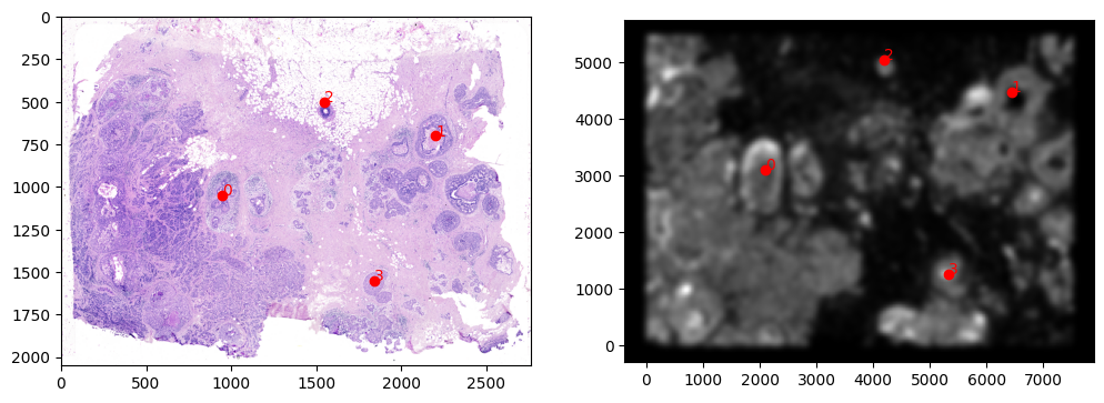
STalign relies on an interative gradient descent to align these two images. This can be somewhat slow. We manually created 3 points that visually mark similar landmarks across the two datasets that we will use to initialize a simple affine alignment from the landmark points.

We can double check that our landmark points look sensible by plotting them along with the rasterized image we created.

# manually make corresponding points
pointsI = np.array([[1050.,950.], [700., 2200.], [500., 1550.], [1550., 1840.]])
pointsJ = np.array([[3108.,2100.], [4480., 6440.], [5040., 4200.], [1260., 5320.]])

# plot
extentJ = STalign.extent_from_x((YJ,XJ))

fig,ax = plt.subplots(1,2)
ax[0].imshow((I.transpose(1,2,0).squeeze()), extent=extentI)
ax[1].imshow((J.transpose(1,2,0).squeeze()), extent=extentJ)

ax[0].scatter(pointsI[:,1],pointsI[:,0], c='red')
ax[1].scatter(pointsJ[:,1],pointsJ[:,0], c='red')
for i in range(pointsI.shape[0]):
    ax[0].text(pointsI[i,1],pointsI[i,0],f'{i}', c='red')
    ax[1].text(pointsJ[i,1],pointsJ[i,0],f'{i}', c='red')

# invert only rasterized image
ax[1].invert_yaxis()

# compute initial affine transformation from points
L,T = STalign.L_T_from_points(pointsI,pointsJ)

From this simple affine transformation based on landmark points, we can already apply the resulting lineared linear transformation (L) and translation (T) to align the single-cell spatial transcriptomics dataset to the H&E staining image. Note that the derived affine transformation is the transformation and translation needed to align the H&E staining image to the single-cell positions. To align the single-cell positions, we will need to invert the linear transformation matrix using linalg.inv and shift in the negative direction by subtracting instead of adding.

print(L)
print(T)
print(L.shape)
print(T.shape)

# note points are as y,x
affine = np.dot(np.linalg.inv(L), [yM - T[0], xM - T[1]])
print(affine.shape)
xMaffine = affine[0,:]
yMaffine = affine[1,:]

# plot
fig,ax = plt.subplots()
ax.scatter(yMaffine,xMaffine,s=1,alpha=0.1)
ax.imshow((I).transpose(1,2,0))

[[-3.65041156  0.06574554]
 [ 0.11365427  3.50866925]]
[ 6832.39702429 -1329.64577839]
(2, 2)
(2,)
(2, 167782)

<matplotlib.image.AxesImage at 0x17f3eb9a0>

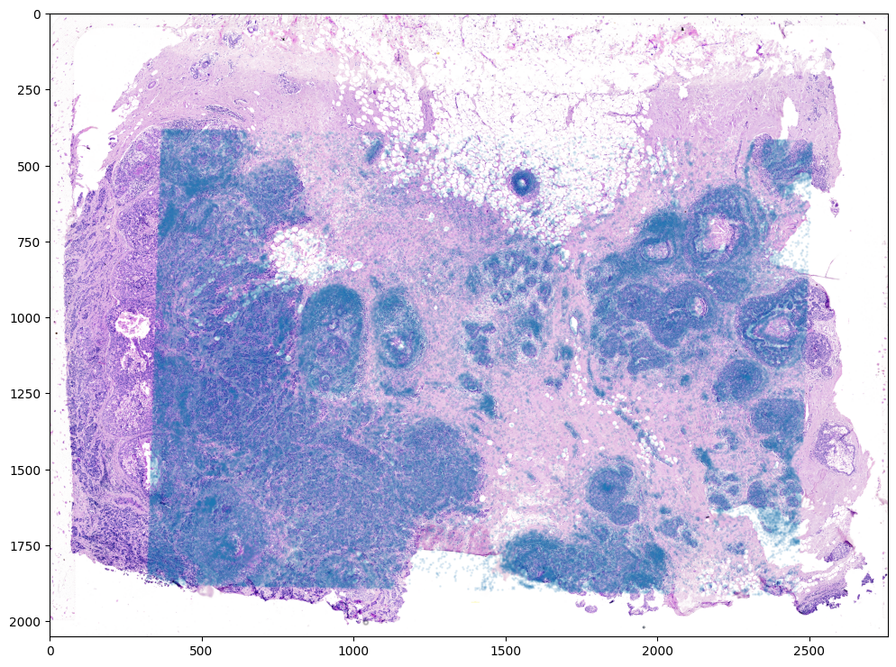
In this case, it seems like either due to the accuracy of our landmark points and/or distortions in the tissue sample introduced during the H&E staining, a simple affine alignment is not sufficient to align the single-cell spatial transcriptomics dataset to the H&E staining image. So we will need to perform non-linear local alignments via LDDMM.

There are many parameters that can be tuned for performing this alignment.

# set device for building tensors
if torch.cuda.is_available():
    torch.set_default_device('cuda:0')
else:
    torch.set_default_device('cpu')

%%time

# run LDDMM
# specify device (default device for STalign.LDDMM is cpu)
if torch.cuda.is_available():
    device = 'cuda:0'
else:
    device = 'cpu'

# keep all other parameters default
params = {'L':L,'T':T,
          'niter':2000,
          'pointsI':pointsI,
          'pointsJ':pointsJ,
          'device':device,
          'sigmaM':0.15,
          'sigmaB':0.10,
          'sigmaA':0.11,
          'epV': 10,
          'muB': torch.tensor([0,0,0]), # black is background in target
          'muA': torch.tensor([1,1,1]) # use white as artifact
          }

out = STalign.LDDMM([YI,XI],I,[YJ,XJ],J,**params)

/Users/kalenclifton/.local/share/virtualenvs/STalign-wXTCUYXW/lib/python3.10/site-packages/torch/functional.py:504: UserWarning: torch.meshgrid: in an upcoming release, it will be required to pass the indexing argument. (Triggered internally at /Users/runner/work/pytorch/pytorch/pytorch/aten/src/ATen/native/TensorShape.cpp:3484.)
  return _VF.meshgrid(tensors, **kwargs)  # type: ignore[attr-defined]
/Users/kalenclifton/STalign/docs/notebooks/../../STalign/STalign.py:1301: UserWarning: Data has no positive values, and therefore cannot be log-scaled.
  axE[2].set_yscale('log')

CPU times: user 1min 48s, sys: 13.6 s, total: 2min 2s
Wall time: 1min 47s

# get necessary output variables
A = out['A']
v = out['v']
xv = out['xv']

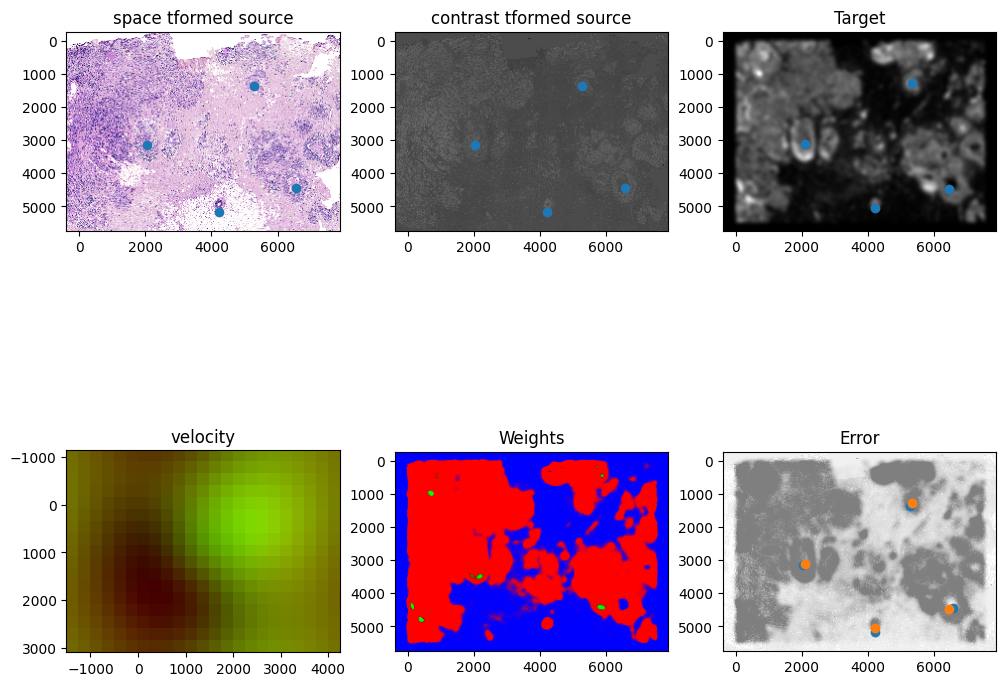
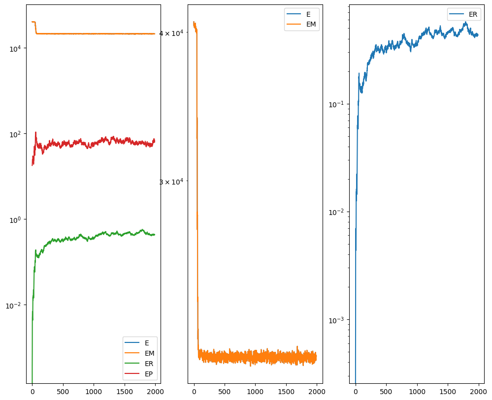
Plots generated throughout the alignment can be used to give you a sense of whether the parameter choices are appropriate and whether your alignment is converging on a solution.

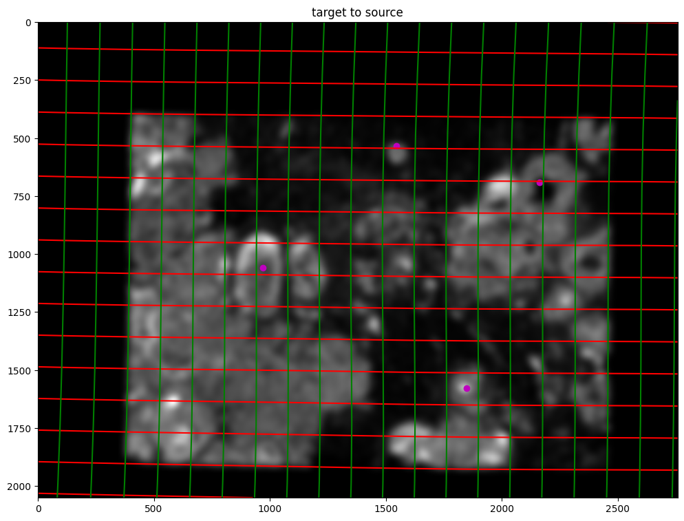
We can also evaluate the resulting alignment by applying the transformation to visualize how our source and target images were deformed to achieve the alignment.

# now transform the points
phi = STalign.build_transform(xv,v,A,XJ=[YI,XI],direction='f')
phiiJ = STalign.transform_image_target_to_source(xv,v,A,[YJ,XJ],J,[YI,XI])
phiipointsJ = STalign.transform_points_target_to_source(xv,v,A,pointsJ)

#switch tensor from cuda to cpu for plotting with numpy
if phi.is_cuda:
    phi = phi.cpu()
if phiiJ.is_cuda:
    phiiJ = phiiJ.cpu()
if phiipointsJ.is_cuda:
    phiipointsJ = phiipointsJ.cpu()

# plot
fig,ax = plt.subplots()

levels = np.arange(-50000,50000,500)

ax.contour(XI,YI,phi[...,0],colors='r',linestyles='-',levels=levels)
ax.contour(XI,YI,phi[...,1],colors='g',linestyles='-',levels=levels)
ax.set_aspect('equal')
ax.set_title('target to source')

ax.imshow(phiiJ.permute(1,2,0),extent=extentI)
ax.scatter(phiipointsJ[:,1].detach(),phiipointsJ[:,0].detach(),c="m")

/Users/kalenclifton/.local/share/virtualenvs/STalign-wXTCUYXW/lib/python3.10/site-packages/torch/utils/_device.py:62: UserWarning: To copy construct from a tensor, it is recommended to use sourceTensor.clone().detach() or sourceTensor.clone().detach().requires_grad_(True), rather than torch.tensor(sourceTensor).
  return func(*args, **kwargs)

<matplotlib.collections.PathCollection at 0x17e3f1930>

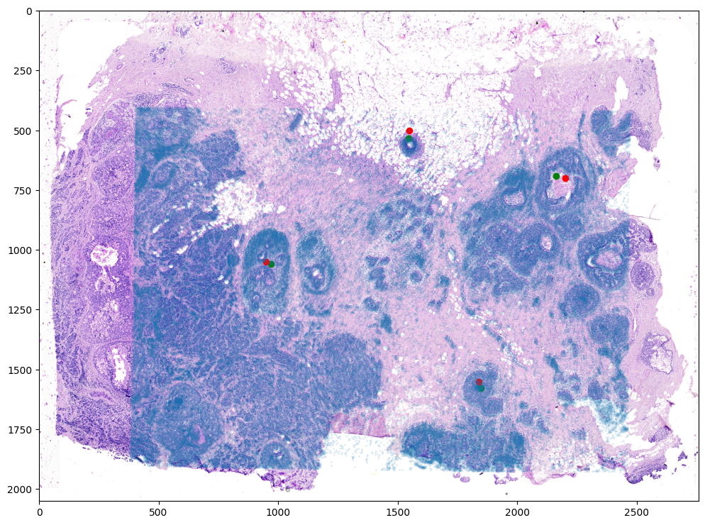
Finally, we can apply our transform to the original sets of single cell centroid positions to achieve their new aligned positions.

# Now apply to points
tpointsJ = STalign.transform_points_target_to_source(xv,v,A,np.stack([yM, xM], -1))

#switch tensor from cuda to cpu for plotting with numpy
if tpointsJ.is_cuda:
    tpointsJ = tpointsJ.cpu()

And we can visualize the results.

# plot

fig,ax = plt.subplots()
ax.imshow((I).transpose(1,2,0),extent=extentI)
ax.scatter(phiipointsJ[:,1].detach(),phiipointsJ[:,0].detach(),c="g")
ax.scatter(pointsI[:,1],pointsI[:,0], c='r')
ax.scatter(tpointsJ[:,1].detach(),tpointsJ[:,0].detach(),s=1,alpha=0.1)

<matplotlib.collections.PathCollection at 0x17f883160>

And save the new aligned positions by appending to our original data using numpy with np.hstack

# save results by appending
results = np.hstack((df, tpointsI.numpy()))

We will finally create a compressed .csv.gz file to create Xenium_Breast_Cancer_Rep1_STalign_to_HE.csv.gz

results.to_csv('../xenium_data/Xenium_Breast_Cancer_Rep1_STalign_to_HE.csv.gz',
               compression='gzip')