Creating RNA-velocity informed 2D embeddings for single cell transcriptomics
VeloViz
![]()
VeloViz creates RNA-velocity-informed low dimensional embeddings for single cell transcriptomics data.

The overall approach is detailed in Atta et. al. Bioinformatics. 2021.
Installation
To install VeloViz, we recommend using remotes:
require(remotes)
remotes::install_github('JEFworks-Lab/veloviz')
VeloViz is also available on Bioconductor:
if (!requireNamespace("BiocManager", quietly = TRUE))
    install.packages("BiocManager")

BiocManager::install("veloviz")
Example
Below is a short example showing how to create a VeloViz embedding on sc-RNAseq data. R objects containing the preprocessed data and velocity models used in this example can be downloaded from Zenodo.
# load packages
library(veloviz)
library(velocyto.R)
# get pancreas scRNA-seq data
download.file("https://zenodo.org/record/4632471/files/pancreas.rda?download=1", destfile = "pancreas.rda", method = "curl")
load("pancreas.rda")
spliced <- pancreas$spliced
unspliced <- pancreas$unspliced
clusters <- pancreas$clusters # cell type annotations
pcs <- pancreas$pcs # PCs used to make other embeddings (UMAP,tSNE..)
#choose colors based on clusters for plotting later
cell.cols <- rainbow(8)[as.numeric(clusters)]
names(cell.cols) <- names(clusters)
# compute velocity using velocyto.R
#cell distance in PC space
cell.dist <- as.dist(1-cor(t(pcs))) # cell distance in PC space
vel <- gene.relative.velocity.estimates(spliced,
unspliced,
kCells = 30,
cell.dist = cell.dist,
fit.quantile = 0.1)
#(or use precomputed velocity object)
# vel <- pancreas$vel
curr <- vel$current
proj <- vel$projected
# build VeloViz graph
veloviz <- buildVeloviz(
curr = curr, proj = proj,
normalize.depth = TRUE,
use.ods.genes = TRUE,
alpha = 0.05,
pca = TRUE,
nPCs = 20,
center = TRUE,
scale = TRUE,
k = 5,
similarity.threshold = 0.25,
distance.weight = 1,
distance.threshold = 0.5,
weighted = TRUE,
seed = 0,
verbose = FALSE
)
# extract VeloViz embedding
emb.veloviz <- veloviz$fdg_coords
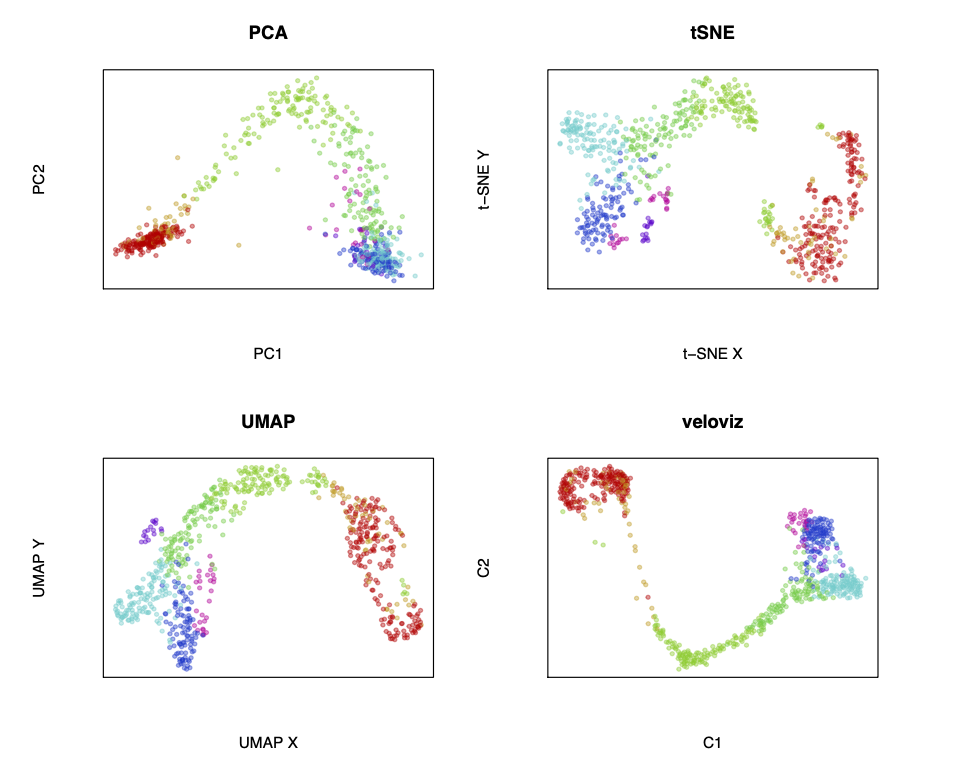
# compare to other embeddings
par(mfrow = c(2,2))
#PCA
emb.pca <- pcs[,1:2]
plotEmbedding(emb.pca, groups=clusters, main='PCA')
#tSNE
set.seed(0)
emb.tsne <- Rtsne::Rtsne(pcs, perplexity=30)$Y
rownames(emb.tsne) <- rownames(pcs)
plotEmbedding(emb.tsne, groups=clusters, main='tSNE',
xlab = "t-SNE X", ylab = "t-SNE Y")
#UMAP
set.seed(0)
emb.umap <- uwot::umap(pcs, min_dist = 0.5)
rownames(emb.umap) <- rownames(pcs)
plotEmbedding(emb.umap, groups=clusters, main='UMAP',
xlab = "UMAP X", ylab = "UMAP Y")
#VeloViz
plotEmbedding(emb.veloviz, groups=clusters[rownames(emb.veloviz)], main='veloviz')
Tutorials
scRNA-seq data preprocessing and visualization using VeloViz
MERFISH cell cycle visualization using VeloViz
Understanding VeloViz parameters
Visualizing the VeloViz graph using UMAP
VeloViz with dynamic velocity estimates from scVelo