VeloViz Parameters

In this tutorial, we will explore the different user-inputted parameters to VeloViz and their effects on the 2D embedding. To do this, we will create a cell cycle simulation with missing intermediates and create VeloViz graphs with various parameter values.

Create simulated cell cycle

set.seed(1)

#make unit circle
t = runif(500,min=0,max=2*pi)
u1 = cos(t)
u2 = sin(t)
traj = cbind(u1,u2)

#OBSERVED
#add noise and uncorrelated dimension
u1 = jitter(u1, amount = 0.25)
u2 = jitter(u2, amount = 0.25)
u3 = rnorm(500)
obs = cbind(u1,u2,u3)

#order by pseduotime
traj = traj[order(t),]
obs = obs[order(t),]

#color by pseudotime
col = colorRampPalette(c(rainbow(10)))(nrow(obs))
labels <- paste0('cell', 1:nrow(obs))
rownames(traj) = labels
rownames(obs) = labels

par(mfrow = c(2,2))
plot(traj, col = col, main = "trajectory")
plot(obs[,1:2], col = col,main = "observed")

#PROJECTED
#rotate by angle a
a = 0.1*pi
exp.u1 = cos(a)*obs[,1] - sin(a)*obs[,2]
exp.u2 = sin(a)*obs[,1] + cos(a)*obs[,2]
set.seed(1)
exp.u3 = rnorm(500)
exp = cbind(exp.u1,exp.u2,exp.u3)
rownames(exp) = labels

plot(exp[,1:2],col = col, main = "expected")
plot(obs[,1:2],col=col, pch=16)
points(exp[,1:2],col=col)
arrows(obs[,1],obs[,2],exp[,1],exp[,2])

Non-velocity based embedding on current expression

pca = RSpectra::svds(A = obs, k=3,
                     opts = list(center = TRUE, scale = TRUE,
                                 maxitr = 2000, tol = 1e-10))
var = pca$d
pcs = pca$u
rownames(pcs) = labels

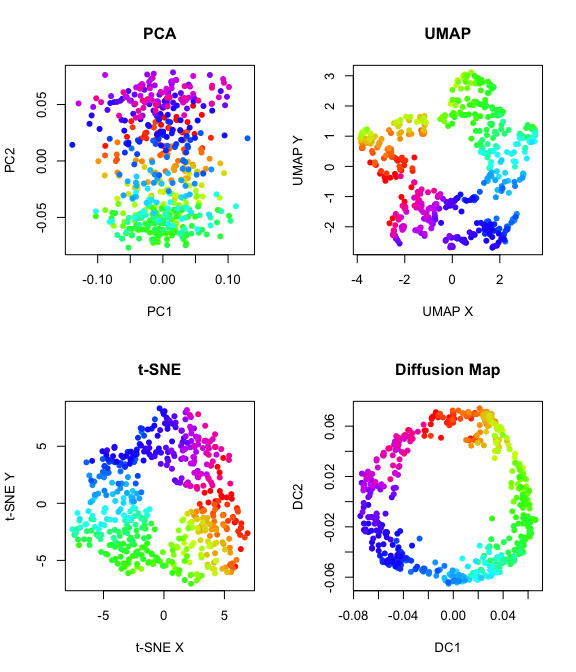
par(mfrow = c(2,2))
#PCA
emb.pca = pcs[,1:2]
plot(emb.pca, pch=16, main = "PCA", xlab = 'PC1', ylab = 'PC2', col = col)

#UMAP
set.seed(1)
emb.umap = uwot::umap(pcs, n_neighbors = 100L)
plot(emb.umap,pch=16, main = "UMAP", xlab = 'UMAP X', ylab = 'UMAP Y',col = col)

#tSNE
set.seed(1)
emb.tsne = Rtsne::Rtsne(pcs,
                        is_distance = FALSE, perplexity = 100,
                        pca = FALSE, num_threads =1, verbose = FALSE)$Y
plot(emb.tsne,pch=16, main = "t-SNE", xlab = 't-SNE X', ylab = 't-SNE Y',col=col)

#diffusion map
set.seed(1)
diffmap = destiny::DiffusionMap(pcs, k=50)
emb.diffmap = destiny::eigenvectors(diffmap)[,1:2]
plot(emb.diffmap,pch=16, main = "Diffusion Map", xlab = 'DC1', ylab = 'DC2',col=col)

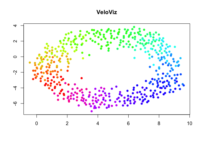
VeloViz Embedding

#, fig.width=7,fig.height=7
set.seed(1) # fig.width=6, fig.height=7
g = graphViz(observed = t(obs), projected = t(exp),
             k = 30, distance_metric = "L2", similarity_metric = "cosine",
             distance_weight = 1, distance_threshold = 1, similarity_threshold = 0.25,
             weighted = TRUE, remove_unconnected = TRUE,
             cell.colors = col, title = "VeloViz",
             plot = FALSE, return_graph = TRUE)
emb.veloviz = g$fdg_coords
plot(emb.veloviz, pch = 16, main = "VeloViz", xlab = '', ylab = '',col=col)

Incomplete Cycle

set.seed(1)

#make unit circle
t = runif(500,min=0,max=2*pi)
u1 = cos(t)
u2 = sin(t)
traj = cbind(u1,u2)

#OBSERVED
#add noise and uncorrelated dimension
u1 = jitter(u1, amount = 0.25)
u2 = jitter(u2, amount = 0.25)
u3 = rnorm(500)
obs = cbind(u1,u2,u3)

#order by pseduotime
traj = traj[order(t),]
obs = obs[order(t),]

#color by pseudotime
col = colorRampPalette(c(rainbow(10)))(nrow(obs))
labels <- paste0('cell', 1:nrow(obs))
rownames(traj) = labels
rownames(obs) = labels
names(col) = labels

#PROJECTED
#rotate by angle a
a = 0.1*pi
exp.u1 = cos(a)*obs[,1] - sin(a)*obs[,2]
exp.u2 = sin(a)*obs[,1] + cos(a)*obs[,2]
set.seed(1)
exp.u3 = rnorm(500)
exp = cbind(exp.u1,exp.u2,exp.u3)
rownames(exp) = labels

#remove cells
cells.keep <- setdiff(labels, paste0('cell', 1:100))
# cells.keep

labels <- labels[which(labels %in% cells.keep)]
obs.missing <- obs[cells.keep,]
exp.missing = exp[cells.keep,]
traj.missing = traj[cells.keep,]
col = col[cells.keep]

par(mfrow = c(2,2))
plot(traj.missing, col = col, main = "trajectory", pch = 16)
plot(obs.missing[,1:2], col = col,main = "observed", pch = 16)
plot(exp.missing[,1:2],col = col, main = "expected")
plot(obs.missing[,1:2],col=col, pch=16)
points(exp.missing[,1:2],col=col)
arrows(obs.missing[,1],obs.missing[,2],exp.missing[,1],exp.missing[,2])

# cells.before = ((traj[1,]>0.5)&(traj[2,]<0))
# cells.after = ((traj[1,]>0.5)&(traj[2,]>0))

cells.before = labels %in% paste0('cell', 470:500)
cells.after = labels %in% paste0('cell', 101:130)

# par(mfrow = c(1,1))
# plot(obs.missing[,1:2],col=col, pch=16)
# points(obs.missing[cells.before,], pch = 4,col = "dark red",cex = 1.5)
# points(obs.missing[cells.after,],pch = 4,col = "dark red",cex = 1.5)

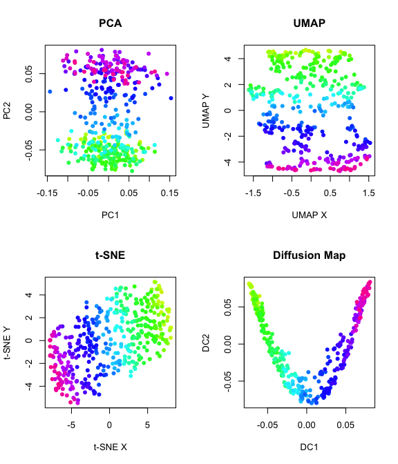
pca = RSpectra::svds(A = obs.missing, k=3,
                     opts = list(center = TRUE, scale = TRUE,
                                 maxitr = 2000, tol = 1e-10))
var = pca$d
pcs = pca$u
rownames(pcs) = labels

par(mfrow = c(2,2))
#PCA
emb.pca = pcs[,1:2]
plot(emb.pca, pch=16, main = "PCA", xlab = 'PC1', ylab = 'PC2', col = col)

#UMAP
set.seed(1)
emb.umap = uwot::umap(pcs, n_neighbors = 100L)
plot(emb.umap,pch=16, main = "UMAP", xlab = 'UMAP X', ylab = 'UMAP Y',col = col)

#tSNE
set.seed(1)
emb.tsne = Rtsne::Rtsne(pcs,
                        is_distance = FALSE, perplexity = 100, pca = FALSE,
                        num_threads =1, verbose = FALSE)$Y
plot(emb.tsne,pch=16, main = "t-SNE", xlab = 't-SNE X', ylab = 't-SNE Y',col=col)

#diffusion map
set.seed(1)
diffmap = destiny::DiffusionMap(pcs, k=50)
emb.diffmap = destiny::eigenvectors(diffmap)[,1:2]
plot(emb.diffmap,pch=16, main = "Diffusion Map", xlab = 'DC1', ylab = 'DC2',col=col)

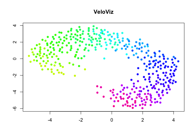
k = 30
distance.weight = 1
distance.threshold = 1
similarity.threshold = 0


set.seed(1)
g = graphViz(observed = t(obs.missing), projected = t(exp.missing),
             k = k, distance_metric = "L2", similarity_metric = "cosine",
             distance_weight = distance.weight, distance_threshold = distance.threshold,
             similarity_threshold = similarity.threshold, weighted = TRUE,
             remove_unconnected = TRUE,
             cell.colors = col, title = "VeloViz",
             plot = FALSE, return_graph = TRUE)
emb.veloviz = g$fdg_coords
plot(emb.veloviz, pch = 16, main = "VeloViz", xlab = '', ylab = '',col=col)

Changing VeloViz Parameters

To understand the effect of each of the parameters, let’s first go through how the VeloViz graph is built to see where each of the parameters comes into play:

Once we have the current and projected transcriptional states in PC space, VeloViz calculates a composite distance for each cell pair. This composite distance has two components: a PC distance component, and a velocity similarity component. If we’re considering the composite distance from Cell A to Cell B, the PC distance component measures how close a Cell A’s projected state is to Cell B. The velocity similarity component measures how similar Cell A’s velocity vector is to the vector representing the transition from Cell A to Cell B.

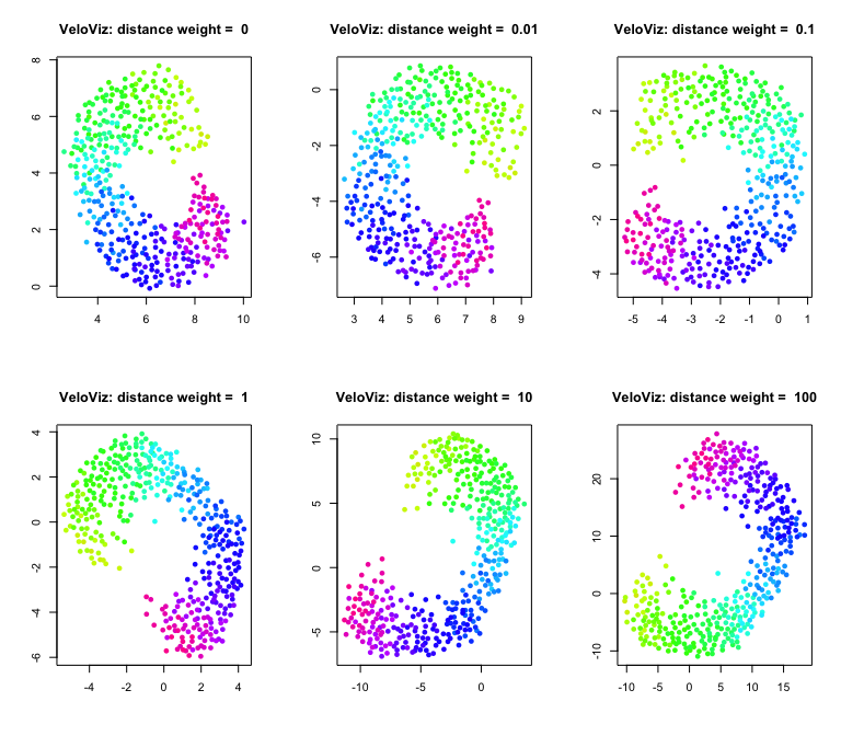
With these composite distances VeloViz creates a k-nearest neighbor graph by assigning k edges from each cell to the k cells with the minimum composite distances. These edges will have a weight corresponding to the composite distance if weighted = TRUE. We can change the relative importance of these two components by changing the distance_weight parameter. Setting distance_weight to 0, results in a graph that only uses velocity similarity to assign edges. Larger values of distance_weight place increasing relative importance on the PC distance component.

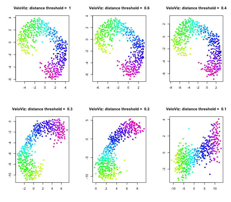
After assigning k out-edges to each cell, VeloViz removes some of these edges based on two threshold parameters, distance_threshold and similarity_threshold. The distance_threshold is a quantile threshold for the PC distance components of the composite distances. For example, setting distance_threshold = 0.2 means that any edges where the PC distance component is not in the smallest 20% of PC distances will be removed from the graph; distance_threshold = 1 includes all edges and does not prune based on distance. Note here that this is 20% of all computed PC distances, not just those in the k-nearest neighbor graph. 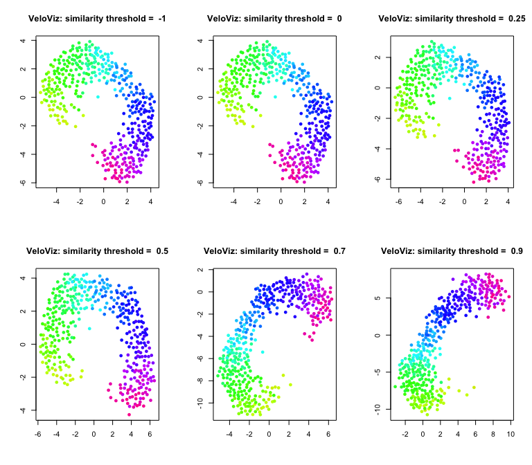The similarity_threshold specifies the minimum cosine similarity between the velocity vector and the cell transition vector for an edge to be included. For example, setting similarity_threshold = 0 removes any edges where the velocity and cell transition vectors are orthogonal or less similar; similarity_threshold = -1 includes all edges and does not prune based on similarity.

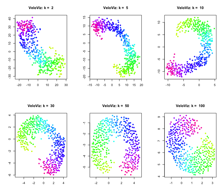
K: Number of nearest neighbors

Now let’s explore how changing the VeloViz parameters changes the embedding, starting with k:

par(mfrow = c(2,3))
ks = c(2,5,10,30,50,100)

distance.weight = 1
distance.threshold = 1
similarity.threshold = 0

for (k in ks) {

  set.seed(1)
  g = graphViz(observed = t(obs.missing), projected = t(exp.missing),
               k = k, distance_metric = "L2", similarity_metric = "cosine",
               distance_weight = distance.weight, distance_threshold = distance.threshold,
               similarity_threshold = similarity.threshold, weighted = TRUE,
               remove_unconnected = TRUE,
               cell.colors = col, title = "VeloViz",
               plot = FALSE, return_graph = TRUE)
  emb.veloviz = g$fdg_coords
  plot(emb.veloviz, pch = 16, main = paste("VeloViz: k = ",k), xlab = '', ylab = '',col=col)

}

Distance weight:

par(mfrow = c(2,3))
dws = c(0,0.01,0.1,1,10,100)

k = 30
distance.threshold = 1
similarity.threshold = 0

for (distance.weight in dws){

  set.seed(1)
  g = graphViz(observed = t(obs.missing), projected = t(exp.missing),
               k = k, distance_metric = "L2", similarity_metric = "cosine",
               distance_weight = distance.weight, distance_threshold = distance.threshold,
               similarity_threshold = similarity.threshold, weighted = TRUE,
               remove_unconnected = TRUE,
               cell.colors = col, title = "VeloViz",
               plot = FALSE, return_graph = TRUE)
  emb.veloviz = g$fdg_coords
  plot(emb.veloviz, pch = 16, main = paste("VeloViz: distance weight = ",distance.weight), xlab = '', ylab = '',col=col)

}

Distance threshold:

par(mfrow = c(2,3))
dts = c(1,0.6,0.4,0.3,0.2,0.1)

k = 30
distance.weight = 1
similarity.threshold = 0

for (distance.threshold in dts){

  set.seed(1)
  g = graphViz(observed = t(obs.missing), projected = t(exp.missing),
               k = k, distance_metric = "L2", similarity_metric = "cosine",
               distance_weight = distance.weight, distance_threshold = distance.threshold,
               similarity_threshold = similarity.threshold, weighted = TRUE,
               remove_unconnected = TRUE,
               cell.colors = col, title = "VeloViz",
               plot = FALSE, return_graph = TRUE)
  emb.veloviz = g$fdg_coords
  plot(emb.veloviz, pch = 16, main = paste("VeloViz: distance threshold = ",distance.threshold), xlab = '', ylab = '',col=col)

}

Similarity threshold:

par(mfrow = c(2,3))
sts = c(-1,0,0.25,0.5,0.7,0.9)

k = 30
distance.weight = 1
distance.threshold = 1

for (similarity.threshold in sts){

  set.seed(1)
  g = graphViz(observed = t(obs.missing), projected = t(exp.missing),
               k = k, distance_metric = "L2", similarity_metric = "cosine",
               distance_weight = distance.weight, distance_threshold = distance.threshold,
               similarity_threshold = similarity.threshold, weighted = TRUE,
               remove_unconnected = TRUE,
               cell.colors = col, title = "VeloViz",
               plot = FALSE, return_graph = TRUE)
  emb.veloviz = g$fdg_coords
  plot(emb.veloviz, pch = 16, main = paste("VeloViz: similarity threshold = ",similarity.threshold), xlab = '', ylab = '',col=col)

}