Creating RNA-velocity informed 2D embeddings for single cell transcriptomics
Visualization using VeloViz
In this tutorial, we will compare the velocity-informed 2D embedding created by VeloViz to other commonly used embeddings. We will go through the workflow needed to generate the VeloViz visualization using the pancreas endocrinogenesis dataset as an example. We will also compare results with VeloViz and other embeddings when some intermediate cells in the developmental trajectory are missing.
Preprocessing
Inputs to VeloViz are the scores in PCA space of the current and
projected transcriptional states, which we get here by calculating RNA
velocity using velocyto.
To get current and projected PC scores from raw counts, we first follow
standard filtering, normalization, and dimensional reduction steps and
then calculate velocity. (Steps 1-3 can be skipped by downloading the preprocessed example data from Zenodo - see 3*).
library(veloviz)
library(reticulate)
library(velocyto.R)
0.) Get Data:
#getting pancreas data from scVelo
scv = import("scvelo")
adata = scv$datasets$pancreas()

#extract spliced, unspliced counts
spliced <- as.matrix(Matrix::t(adata$layers['spliced']))
unspliced <- as.matrix(Matrix::t(adata$layers['unspliced']))
cells <- adata$obs_names$values
genes <- adata$var_names$values
colnames(spliced) <- colnames(unspliced) <- cells
rownames(spliced) <- rownames(unspliced) <- genes

#clusters
clusters <- adata$obs$clusters
names(clusters) <- adata$obs_names$values

#subsample to make things faster
set.seed(0)
good.cells <- sample(cells, length(cells)/5)
spliced <- spliced[,good.cells]
unspliced <- unspliced[,good.cells]
clusters <- clusters[good.cells]

dim(spliced)
dim(unspliced)
1.) Filter good genes
#keep genes with >10 total counts
good.genes = genes[rowSums(spliced) > 10 & rowSums(unspliced) > 10]
spliced = spliced[good.genes,]
unspliced = unspliced[good.genes,]

dim(spliced)
dim(unspliced)
2.) Normalize
counts = spliced + unspliced # use combined spliced and unspliced counts
cpm = normalizeDepth(counts) # normalize to counts per million
lognorm = log10(varnorm + 1) # log normalize
3.) Reduce Dimensions
After filtering and normalizing, we reduce dimensions, and calculate
cell-cell distance in PC space. This distance will be used to compute
velocity.
#PCA on centered and scaled expression of overdispersed genes
pcs = reduceDimensions(lognorm, center = TRUE, scale = TRUE, nPCs = 50)

#cell distance in PC space
cell.dist = as.dist(1-cor(t(pcs))) # cell distance in PC space
3*) Download preprocessed data from Zenodo.
# get pancreas scRNA-seq data
download.file("https://zenodo.org/record/4632471/files/pancreas.rda?download=1", destfile = "pancreas.rda", method = "curl")
load("pancreas.rda")

spliced = pancreas$spliced
unspliced = pancreas$unspliced
clusters = pancreas$clusters
pcs = pancreas$pcs

#choose colors based on clusters for plotting later
cell.cols = rainbow(8)[as.numeric(clusters)]
names(cell.cols) = names(clusters)
Velocity
4.) Calculate velocity
Next, we compute velocity from spliced and unspliced counts and
cell-cell distances using velocyto. This will give us the current and
projected transcriptional states.
#cell distance in PC space
cell.dist = as.dist(1-cor(t(pcs))) # cell distance in PC space

vel = gene.relative.velocity.estimates(spliced,
                                       unspliced,
                                       kCells = 30,
                                       cell.dist = cell.dist,
                                       fit.quantile = 0.1)

#(or use precomputed velocity object)
# vel = pancreas$vel
5.) Normalize current and projected
Now that we have the current and projected expression, we want to go
through a similar normalization process as we did with the raw counts
and then reduce dimensions in PCA. Steps 5-7 can be done together using
the buildVeloviz function (see 7*).
curr = vel$current
proj = vel$projected

#normalize depth
curr.norm = normalizeDepth(curr)
proj.norm = normalizeDepth(proj)

#variance stabilize current
curr.varnorm.info = normalizeVariance(curr.norm, details = TRUE)
curr.varnorm = curr.varnorm.info$matnorm

#use same model for projected
scale.factor = curr.varnorm.info$df$scale_factor #gene scale factors
names(scale.factor) = rownames(curr.varnorm.info$df)

m = proj.norm
rmean = Matrix::rowMeans(m) #row mean
sumx = Matrix::rowSums(m)
sumxx = Matrix::rowSums(m^2)
rsd = sqrt((sumxx - 2 * sumx * rmean + ncol(m) * rmean ^ 2) / (ncol(m)-1)) #row sd

proj.varnorm = proj.norm / rsd * scale.factor[names(rsd)]
proj.varnorm = proj.norm[rownames(curr.varnorm),]
6.) Project current and projected into PC space
#log normalize
curr.pca = log10(curr.varnorm + 1)
proj.pca = log10(proj.varnorm + 1)

#mean center
c.rmean = Matrix::rowMeans(curr.pca)
curr.pca = curr.pca - c.rmean
p.rmean = Matrix::rowMeans(proj.pca)
proj.pca = proj.pca - p.rmean

#scale variance
c.sumx = Matrix::rowSums(curr.pca)
c.sumxx = Matrix::rowSums(curr.pca^2)
c.rsd = sqrt((c.sumxx - 2*c.sumx*c.rmean + ncol(curr.pca)*c.rmean^2)/(ncol(curr.pca)-1))
curr.pca = curr.pca/c.rsd

p.sumx = Matrix::rowSums(proj.pca)
p.sumxx = Matrix::rowSums(proj.pca^2)
p.rsd = sqrt((p.sumxx - 2*p.sumx*p.rmean + ncol(proj.pca)*p.rmean^2)/(ncol(proj.pca)-1))
proj.pca = proj.pca/p.rsd

#PCA
pca = RSpectra::svds(A = Matrix::t(curr.pca), k=20,
                     opts = list(
                       center = FALSE, ## already done
                       scale = FALSE, ## already done
                       maxitr = 2000,
                       tol = 1e-10))

#scores of current and projected
curr.scores = Matrix::t(curr.pca) %*% pca$v[,1:10]
proj.scores = Matrix::t(proj.pca) %*% pca$v[,1:10]
VeloViz
7.) Build graph using VeloViz
Now we can use the PC projections of the current and projected
transcriptional states to build the VeloViz graph. To build the graph,
we have to specify multiple parameters that control the features of the
graph:
k: how many out-edges each cell can have
similarity_threshold: cosine similarity threshold specifying how
similar the velocity and cell transition vectors have to be for an
out-edge to be included
distance_weight: weight for distance component of composite
distance - with large weights, graph will prioritize linking cells where
projected states and neighbors are close in PC space; with small
weights, graph will prioritize linking cells where velocity and cell
transition vectors are most similar
distance_threshold: quantile threshold specifying minimum distance
in PC space between projected state and neighbor for out-edge to be
included - e.g. a distance threshold of 0.2 means that any edges where
the distance component is not in the smallest 20% of distances in PC
space will be removed from the graph
weighted: whether to use composite distance to determine graph
edge weights (TRUE) or to assign all edges equal weights (FALSE)
#VeloViz graph parameters
k = 5
similarity.threshold = 0.25
distance.weight = 1
distance.threshold = 0.5
weighted = TRUE
#build graph
set.seed(0)
veloviz = graphViz(t(curr.scores), t(proj.scores), k,
cell.colors=NA,
similarity_threshold=similarity.threshold,
distance_weight = distance.weight,
distance_threshold = distance.threshold,
weighted = weighted,
plot = FALSE,
return_graph = TRUE)
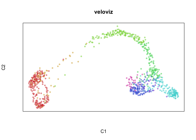
emb.veloviz = veloviz$fdg_coords
plotEmbedding(emb.veloviz, groups=clusters[rownames(emb.veloviz)], main='veloviz')
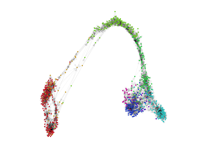
par(mfrow=c(1,1), mar=rep(1,4))
g = plotVeloviz(veloviz, clusters=clusters[rownames(emb.veloviz)], seed=0, verbose=TRUE)
7*) Build VeloViz graph from current and projected using buildVeloviz
curr = vel$current
proj = vel$projected

veloviz = buildVeloviz(
  curr = curr, proj = proj,
  normalize.depth = TRUE,
  use.ods.genes = TRUE,
  alpha = 0.05,
  pca = TRUE,
  nPCs = 20,
  center = TRUE,
  scale = TRUE,
  k = 5,
  similarity.threshold = 0.25,
  distance.weight = 1,
  distance.threshold = 0.5,
  weighted = TRUE,
  seed = 0,
  verbose = FALSE
)

emb.veloviz = veloviz$fdg_coords
plotEmbedding(emb.veloviz, groups=clusters[rownames(emb.veloviz)], main='veloviz')
par(mfrow=c(1,1), mar=rep(1,4))
g = plotVeloviz(veloviz, clusters=clusters[rownames(emb.veloviz)], seed=0, verbose=TRUE)
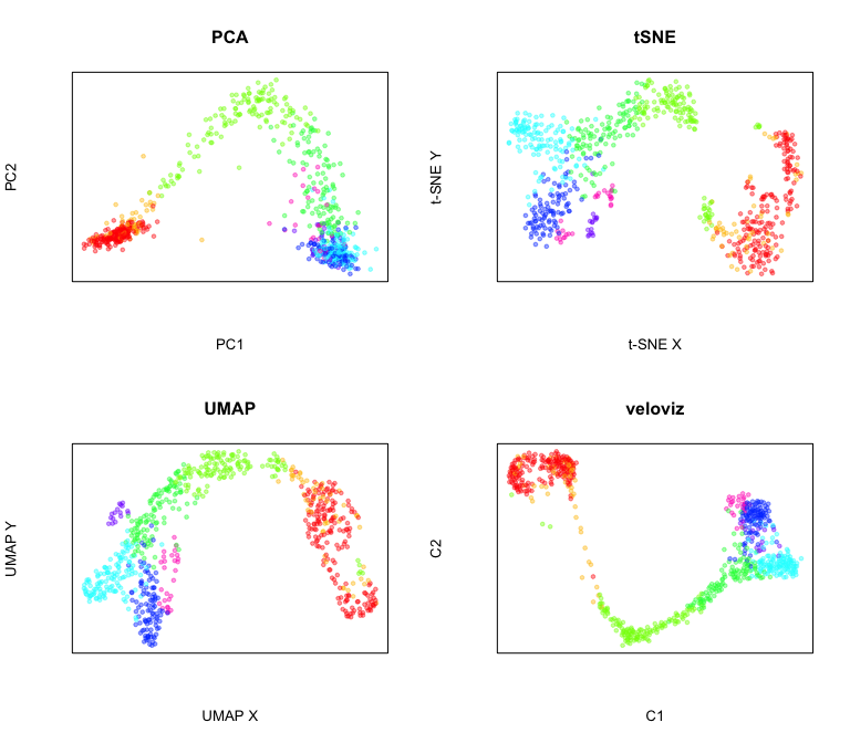
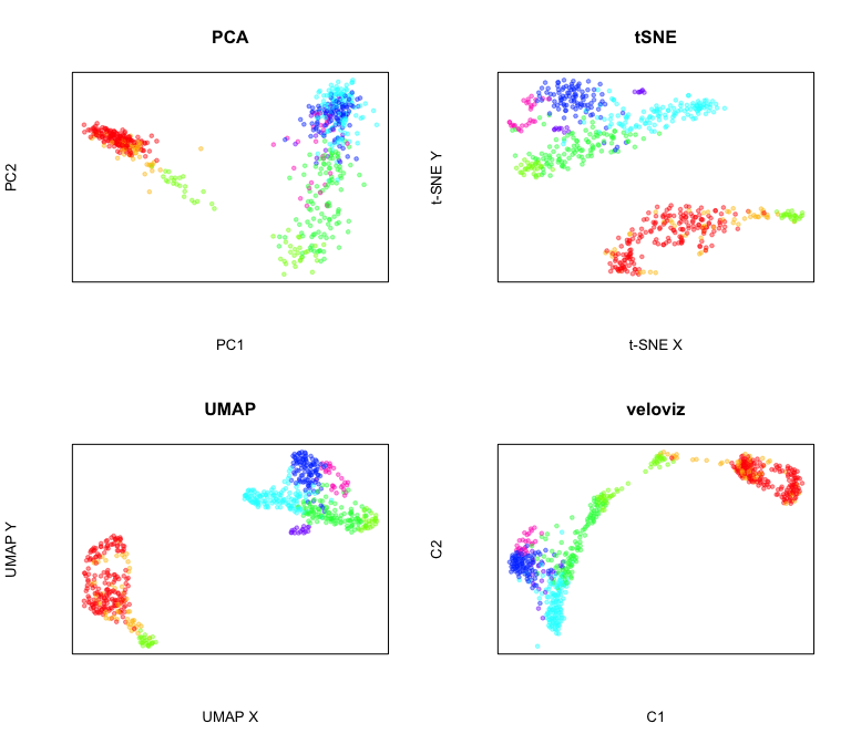
Compare to other embeddings
par(mfrow = c(2,2))

#PCA
emb.pca = pcs[,1:2]
plotEmbedding(emb.pca, colors = cell.cols, main='PCA',
              xlab = "PC1", ylab = "PC2")

#tSNE
set.seed(0)
emb.tsne = Rtsne::Rtsne(pcs, perplexity=30)$Y
rownames(emb.tsne) = rownames(pcs)
plotEmbedding(emb.tsne, colors = cell.cols, main='tSNE',
              xlab = "t-SNE X", ylab = "t-SNE Y")

##UMAP
set.seed(0)
emb.umap = uwot::umap(pcs, min_dist = 0.5)
rownames(emb.umap) <- rownames(pcs)
plotEmbedding(emb.umap, colors = cell.cols, main='UMAP',
              xlab = "UMAP X", ylab = "UMAP Y")

#veloviz
plotEmbedding(emb.veloviz, colors = cell.cols[rownames(emb.veloviz)], main='veloviz')
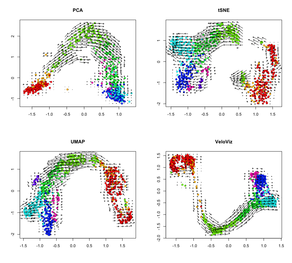
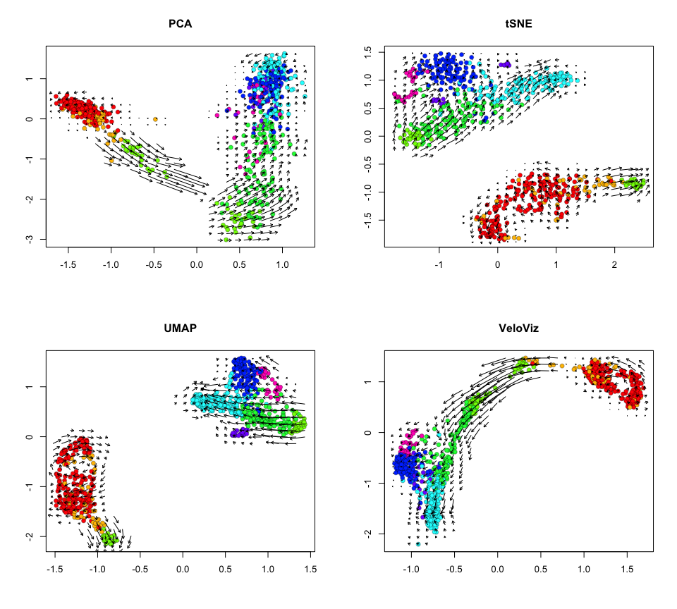
Now let’s project velocity inferred from velocyto.R onto these
embeddings.
par(mfrow = c(2,2))

show.velocity.on.embedding.cor(scale(emb.pca), vel,
                               n = 50,
                               scale='sqrt',
                               cex=1, arrow.scale=1, show.grid.flow=TRUE,
                               min.grid.cell.mass=0.5, grid.n=30, arrow.lwd=1, do.par = FALSE,
                               cell.colors=cell.cols, main='PCA')
show.velocity.on.embedding.cor(scale(emb.tsne), vel,
                               n = 50,
                               scale='sqrt',
                               cex=1, arrow.scale=1, show.grid.flow=TRUE,
                               min.grid.cell.mass=0.5, grid.n=30, arrow.lwd=1,do.par = FALSE,
                               cell.colors=cell.cols, main='tSNE')
show.velocity.on.embedding.cor(scale(emb.umap), vel,
                               n = 50,
                               scale='sqrt',
                               cex=1, arrow.scale=1, show.grid.flow=TRUE,
                               min.grid.cell.mass=0.5, grid.n=30, arrow.lwd=1,do.par = FALSE,
                               cell.colors=cell.cols, main='UMAP')
show.velocity.on.embedding.cor(scale(emb.veloviz), vel,
                               n = 50,
                               scale='sqrt',
                               cex=1, arrow.scale=1, show.grid.flow=TRUE,
                               min.grid.cell.mass=0.5, grid.n=30, arrow.lwd=1,do.par = FALSE,
                               cell.colors=cell.cols, main='VeloViz')
Visualization with missing intermediates using VeloViz
Download data with missing intermediates: this is the same dataset as above but missing a proportion of Ngn3 high EP cells
# get data
download.file("https://zenodo.org/record/4632471/files/pancreasWithGap.rda?download=1", destfile = "pancreasWithGap.rda", method = "curl")
load("pancreasWithGap.rda")

spliced = pancreasWithGap$spliced
unspliced = pancreasWithGap$unspliced
clusters = pancreasWithGap$clusters
pcs = pancreasWithGap$pcs

#choose colors based on clusters for plotting later
cell.cols = rainbow(8)[as.numeric(clusters)]
names(cell.cols) = names(clusters)
Compute velocity
#cell distance in PC space
cell.dist = as.dist(1-cor(t(pcs))) # cell distance in PC space

vel = gene.relative.velocity.estimates(spliced,
                                       unspliced,
                                       kCells = 30,
                                       cell.dist = cell.dist,
                                       fit.quantile = 0.1)

#(or use precomputed velocity object)
# vel = pancreasWithGap$vel
Create VeloViz embedding
curr = vel$current
proj = vel$projected
veloviz = buildVeloviz(
curr = curr, proj = proj,
normalize.depth = TRUE,
use.ods.genes = TRUE,
alpha = 0.05,
pca = TRUE,
nPCs = 20,
center = TRUE,
scale = TRUE,
k = 5,
similarity.threshold = 0.25,
distance.weight = 1,
distance.threshold = 0.5,
weighted = TRUE,
seed = 0,
verbose = FALSE
)
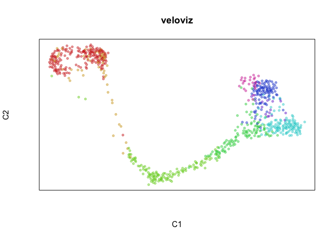
emb.veloviz = veloviz$fdg_coords
plotEmbedding(emb.veloviz, groups=clusters[rownames(emb.veloviz)], main='veloviz')
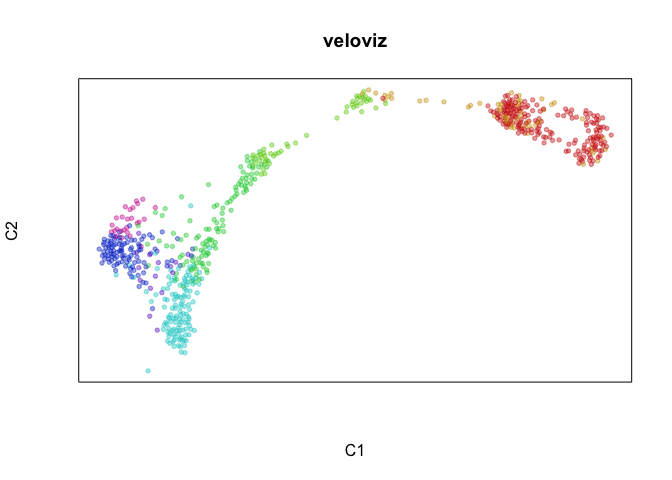
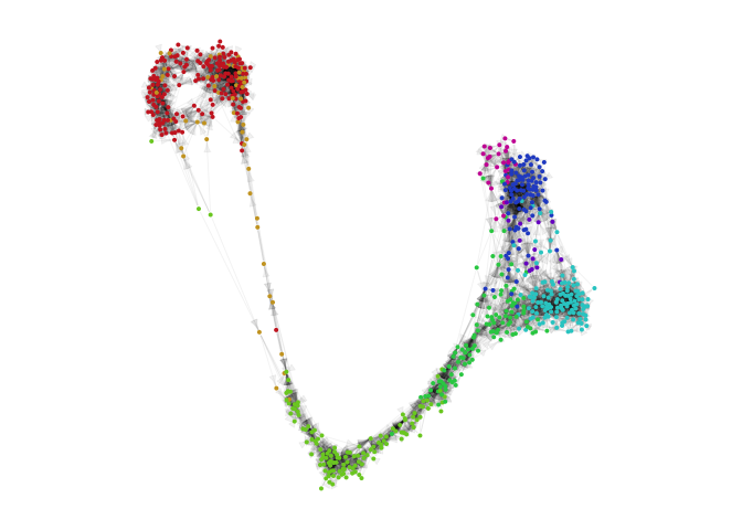
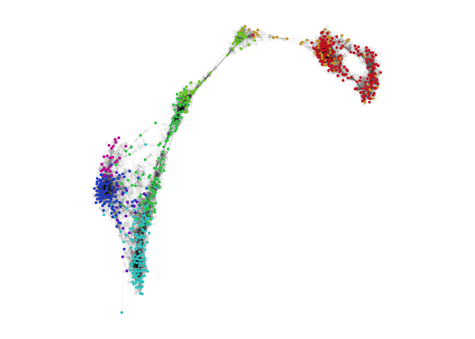
par(mfrow=c(1,1), mar=rep(1,4))
g = plotVeloviz(veloviz, clusters=clusters[rownames(emb.veloviz)], seed=0, verbose=TRUE)
Compare to other embeddings
par(mfrow = c(2,2))

#PCA
emb.pca = pcs[,1:2]
plotEmbedding(emb.pca, colors = cell.cols, main='PCA')

#tSNE
set.seed(0)
emb.tsne = Rtsne::Rtsne(pcs, perplexity=30)$Y
rownames(emb.tsne) = rownames(pcs)
plotEmbedding(emb.tsne, colors = cell.cols, main='tSNE',
              xlab = "t-SNE X", ylab = "t-SNE Y")

##UMAP
set.seed(0)
emb.umap = uwot::umap(pcs, min_dist = 0.5)
rownames(emb.umap) <- rownames(pcs)
plotEmbedding(emb.umap, colors = cell.cols, main='UMAP',
              xlab = "UMAP X", ylab = "UMAP Y")

#veloviz
plotEmbedding(emb.veloviz, colors = cell.cols[rownames(emb.veloviz)], main='veloviz')
Now let’s project velocity inferred from velocyto.R onto these
embeddings.
par(mfrow = c(2,2))

show.velocity.on.embedding.cor(scale(emb.pca), vel,
                               n = 50,
                               scale='sqrt',
                               cex=1, arrow.scale=1, show.grid.flow=TRUE,
                               min.grid.cell.mass=0.5, grid.n=30, arrow.lwd=1, do.par = FALSE,
                               cell.colors=cell.cols, main='PCA')
show.velocity.on.embedding.cor(scale(emb.tsne), vel,
                               n = 50,
                               scale='sqrt',
                               cex=1, arrow.scale=1, show.grid.flow=TRUE,
                               min.grid.cell.mass=0.5, grid.n=30, arrow.lwd=1,do.par = FALSE,
                               cell.colors=cell.cols, main='tSNE')
show.velocity.on.embedding.cor(scale(emb.umap), vel,
                               n = 50,
                               scale='sqrt',
                               cex=1, arrow.scale=1, show.grid.flow=TRUE,
                               min.grid.cell.mass=0.5, grid.n=30, arrow.lwd=1,do.par = FALSE,
                               cell.colors=cell.cols, main='UMAP')
show.velocity.on.embedding.cor(scale(emb.veloviz), vel,
                               n = 50,
                               scale='sqrt',
                               cex=1, arrow.scale=1, show.grid.flow=TRUE,
                               min.grid.cell.mass=0.5, grid.n=30, arrow.lwd=1,do.par = FALSE,
                               cell.colors=cell.cols, main='VeloViz')
Other tutorials
Getting Started
MERFISH cell cycle visualization using VeloViz
Understanding VeloViz parameters
Visualizing the VeloViz graph using UMAP
VeloViz with dynamic velocity estimates from scVelo