Creating RNA-velocity informed 2D embeddings for single cell transcriptomics
Visualizing MERFISH data using VeloViz
In this vignette, we will use VeloViz to create a 2D embedding to visualize MERFISH data collected from U-2 OS cells in culture. Since this data comes from a cell line in culture, we expect the main temporal signal to be progression throught the cell-cycle. We will compare the VeloViz embedding to simply using the first two principal components. We will also compare the results we get when we restrict the input genes. The data used for this example was initially obtained from the Xia et. al., PNAS, 2019. An R object containing the preprocessed example data is available at Zenodo
Load data
MERFISH data from Xia et. al., PNAS, 2019. This data is provided with the VeloViz package. Since this data doesn’t distinguish between spliced and unspliced RNAs, we insteda use cytplasmic and nuclear counts to calculate velocity.
library(veloviz)
library(velocyto.R)

# get MERFISH data
download.file("https://zenodo.org/record/4632471/files/MERFISH.rda?download=1", destfile = "MERFISH.rda", method = "curl")
load("MERFISH.rda")

col <- MERFISH$col #colors based on louvain clusters
pcs <- MERFISH$pcs

cyto <- MERFISH$cyto #cytplasmic counts
nuc <- MERFISH$nuc #nuclear counts
Using all genes
Velocity
cell.dists <- as.dist(1-cor(t(pcs))) #distances in PC space - used for velocity
vel <- velocyto.R::gene.relative.velocity.estimates(as.matrix(cyto),
                                                    as.matrix(nuc), kCells = 30,
                                                    cell.dist = cell.dists,
                                                    fit.quantile = 0.1)


#(or use precomputed velocity)
#vel <- MERFISH$vel

curr <- vel$current
proj <- vel$projected
Build VeloViz embedding
veloviz <-  buildVeloviz(curr = curr, proj = proj,
                         normalize.depth = TRUE,
                         use.ods.genes = FALSE,
                         pca = TRUE, nPCs = 3,
                         center = TRUE, scale = TRUE,
                         k = 50, similarity.threshold = -1,
                         distance.weight = 1, distance.threshold = 1,
                         weighted = TRUE, seed = 0, verbose = FALSE)

emb.veloviz <- veloviz$fdg_coords
Other embeddings
#PCA - we've already computed PCs
emb.pca <- pcs[,1:2]

#t-SNE
set.seed(0)
emb.tsne <- Rtsne::Rtsne(pcs, pca=FALSE)$Y
rownames(emb.tsne) <- rownames(pcs)

#UMAP
set.seed(0)
emb.umap <- uwot::umap(pcs)
rownames(emb.umap) <- rownames(pcs)
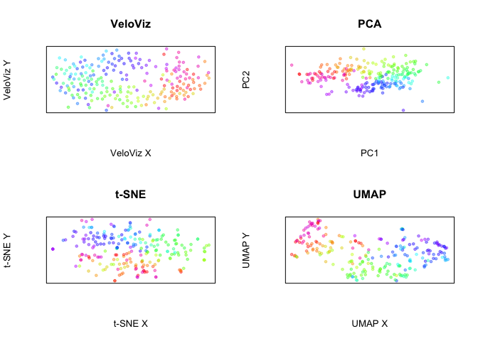
Now, plot all embeddings
par(mfrow = c(2,2))

plotEmbedding(emb.veloviz, colors = col[rownames(emb.veloviz)],
              main = 'VeloViz', xlab = "VeloViz X", ylab = "VeloViz Y")
plotEmbedding(emb.pca, colors = col,
              main = 'PCA', xlab = "PC1", ylab = "PC2")
plotEmbedding(emb.tsne, colors = col,
              main = 't-SNE', xlab = "t-SNE X", ylab = "t-SNE Y")
plotEmbedding(emb.umap, colors = col,
              main = 'UMAP', xlab = "UMAP X", ylab = "UMAP Y")
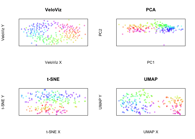
Using GO cell cycle genes
Now let’s compare these embeddings to embeddings created using only cell cycle genes in the GO mitotic cell-cycle gene set.
#GO cell cycle genes (GO:0000278)
# https://www.gsea-msigdb.org/gsea/msigdb/cards/GO_MITOTIC_CELL_CYCLE
cycle.genes.go <- read.csv("GO_0000278.csv",header = FALSE)$V1
cycle.genes.go <- intersect(cycle.genes.go, rownames(nuc)) #GO cell cycle genes that are in MERFISH data

cyto.go <- cyto[cycle.genes.go,]
nuc.go <- nuc[cycle.genes.go,]
Compute new PCs..
all.go <- cyto.go + nuc.go
#normalize and dim red
cpm <- normalizeDepth(all.go)
lognorm <- log10(cpm+1)
pcs.go <- veloviz::reduceDimensions(lognorm, center = T, scale = T)
cell.dist <- as.dist(1-cor(t(pcs.go)))
Velocity
vel.go <- velocyto.R::gene.relative.velocity.estimates(as.matrix(cyto.go),
                                                    as.matrix(nuc.go), kCells = 30,
                                                    cell.dist = cell.dists,
                                                    fit.quantile = 0.1)
curr.go <- vel.go$current
proj.go <- vel.go$projected
Build VeloViz embedding
veloviz.go <-  buildVeloviz(curr = curr.go, proj = proj.go,
                         normalize.depth = TRUE,
                         use.ods.genes = FALSE,
                         pca = TRUE, nPCs = 3,
                         center = TRUE, scale = TRUE,
                         k = 50, similarity.threshold = -1,
                         distance.weight = 1, distance.threshold = 1,
                         weighted = TRUE, seed = 0, verbose = FALSE)

emb.veloviz.go <- veloviz.go$fdg_coords
Other embeddings
#PCA - we've already computed PCs
emb.pca.go <- pcs.go[,1:2]

#t-SNE
set.seed(0)
emb.tsne.go <- Rtsne::Rtsne(pcs.go, pca=FALSE)$Y
rownames(emb.tsne.go) <- rownames(pcs.go)

#UMAP
set.seed(0)
emb.umap.go <- uwot::umap(pcs.go)
rownames(emb.umap.go) <- rownames(pcs.go)
Now, plot all embeddings
par(mfrow = c(2,2))

plotEmbedding(emb.veloviz.go, colors = col[rownames(emb.veloviz.go)],
              main = 'VeloViz', xlab = "VeloViz X", ylab = "VeloViz Y")
plotEmbedding(emb.pca.go, colors = col,
              main = 'PCA', xlab = "PC1", ylab = "PC2")
plotEmbedding(emb.tsne.go, colors = col,
              main = 't-SNE', xlab = "t-SNE X", ylab = "t-SNE Y")
plotEmbedding(emb.umap.go, colors = col,
              main = 'UMAP', xlab = "UMAP X", ylab = "UMAP Y")
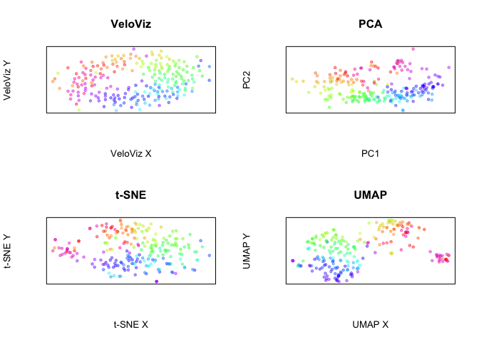
Using genes with cell cycle dependent expression
Xia et. al. identified genes with cell cycle dependent expression. Let’s construct the embeddings with only those genes.
#MERFISH genes exhibiting cell-cycle-dependent expression (Xia et al 2019, Supp Dataset 8)
# https://www.pnas.org/content/116/39/19490
cycle.genes.xia <- read.csv("pnas_sd08.csv",header = TRUE)$Gene
cycle.genes.xia <- intersect(cycle.genes.xia, rownames(nuc)) #genes that are also in MERFISH data

cyto.xia <- cyto[cycle.genes.xia,]
nuc.xia <- nuc[cycle.genes.xia,]
Compute new PCs..
all.xia <- cyto.xia + nuc.xia
#normalize and dim red
cpm <- normalizeDepth(all.xia)
lognorm <- log10(cpm+1)
pcs.xia <- veloviz::reduceDimensions(lognorm, center = T, scale = T)
cell.dist <- as.dist(1-cor(t(pcs.xia)))
Velocity
vel.xia <- velocyto.R::gene.relative.velocity.estimates(as.matrix(cyto.xia),
                                                    as.matrix(nuc.xia), kCells = 30,
                                                    cell.dist = cell.dists,
                                                    fit.quantile = 0.1)
curr.xia <- vel.xia$current
proj.xia <- vel.xia$projected
Build VeloViz embedding
veloviz.xia <-  buildVeloviz(curr = curr.xia, proj = proj.xia,
                         normalize.depth = TRUE,
                         use.ods.genes = FALSE,
                         pca = TRUE, nPCs = 3,
                         center = TRUE, scale = TRUE,
                         k = 50, similarity.threshold = -1,
                         distance.weight = 1, distance.threshold = 1,
                         weighted = TRUE, seed = 0, verbose = FALSE)

emb.veloviz.xia <- veloviz.xia$fdg_coords
Other embeddings
#PCA - we've already computed PCs
emb.pca.xia <- pcs.xia[,1:2]

#t-SNE
set.seed(0)
emb.tsne.xia <- Rtsne::Rtsne(pcs.xia, pca=FALSE)$Y
rownames(emb.tsne.xia) <- rownames(pcs.xia)

#UMAP
set.seed(0)
emb.umap.xia <- uwot::umap(pcs.xia)
rownames(emb.umap.xia) <- rownames(pcs.xia)
Now, plot all embeddings
par(mfrow = c(2,2))

plotEmbedding(emb.veloviz.xia, colors = col[rownames(emb.veloviz.xia)],
              main = 'VeloViz', xlab = "VeloViz X", ylab = "VeloViz Y")
plotEmbedding(emb.pca.xia, colors = col,
              main = 'PCA', xlab = "PC1", ylab = "PC2")
plotEmbedding(emb.tsne.xia, colors = col,
              main = 't-SNE', xlab = "t-SNE X", ylab = "t-SNE Y")
plotEmbedding(emb.umap.xia, colors = col,
              main = 'UMAP', xlab = "UMAP X", ylab = "UMAP Y")
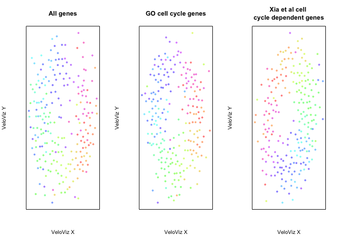
Comparing VeloViz embeddings
VeloViz embeddings constructed with different gene sets
par(mfrow = c(1,3))
plotEmbedding(emb.veloviz, colors = col[rownames(emb.veloviz)],
              main = 'All genes', xlab = "VeloViz X", ylab = "VeloViz Y")
plotEmbedding(emb.veloviz.go, colors = col[rownames(emb.veloviz.go)],
              main = 'GO cell cycle genes', xlab = "VeloViz X", ylab = "VeloViz Y")
plotEmbedding(emb.veloviz.xia, colors = col[rownames(emb.veloviz.xia)],
              main = 'Xia et al cell \ncycle dependent genes', xlab = "VeloViz X", ylab = "VeloViz Y")
Other tutorials
Getting Started
scRNA-seq data preprocessing and visualization using VeloViz
Understanding VeloViz parameters
Visualizing the VeloViz graph using UMAP
VeloViz with dynamic velocity estimates from scVelo