Creating RNA-velocity informed 2D embeddings for single cell transcriptomics
Visualizing the VeloViz graph using UMAP
In this example, we will use Veloviz to produce a velocity-informed 2D embedding and will then pass the computed nearest neighbor data into UMAP. This is useful to users who want to use common algorithms such as t-SNE and UMAP to layout their embedding. We will use the pancreas endocrinogenesis dataset in this example.
First, load libraries:
library(veloviz)
library(velocyto.R)
library(uwot)
Next, get preprocessed example data Zenodo:
# get pancreas scRNA-seq data
download.file("https://zenodo.org/record/4632471/files/pancreas.rda?download=1", destfile = "pancreas.rda", method = "curl")
load("pancreas.rda")

spliced = pancreas$spliced
unspliced = pancreas$unspliced
clusters = pancreas$clusters
pcs = pancreas$pcs

#choose colors based on clusters for plotting later
cell.cols = rainbow(8)[as.numeric(clusters)]
names(cell.cols) = names(clusters)
Compute velocity:
#cell distance in PC space
cell.dist = as.dist(1-cor(t(pcs))) # cell distance in PC space

vel = gene.relative.velocity.estimates(spliced,
                                       unspliced,
                                       kCells = 30,
                                       cell.dist = cell.dist,
                                       fit.quantile = 0.1)

 #(or use precomputed velocity object)
 # vel = pancreas$vel
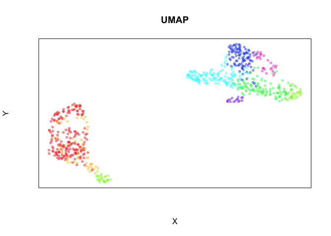
Embed using UMAP with PCs as inputs:
set.seed(0)
emb.umap <- uwot::umap(pcs, min_dist = 0.5)
rownames(emb.umap) <- rownames(pcs)

plotEmbedding(emb.umap, colors = cell.cols,
              main = 'UMAP', xlab = "X", ylab = "Y")
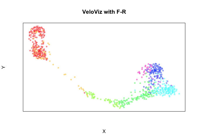
Now, build VeloViz graph:
curr <- vel$current
proj <- vel$projected

veloviz.graph <- buildVeloviz(
  curr = curr,
  proj = proj,
  normalize.depth = TRUE,
  use.ods.genes = TRUE,
  alpha = 0.05,
  pca = TRUE,
  nPCs = 20,
  center = TRUE,
  scale = TRUE,
  k = 20,
  similarity.threshold = 0,
  distance.weight = 1,
  distance.threshold = 0,
  weighted = TRUE,
  seed = 0,
  verbose = FALSE
)

emb.veloviz <- veloviz.graph$fdg_coords
plotEmbedding(emb.veloviz, colors = cell.cols,
              main = 'VeloViz with F-R', xlab = "X", ylab = "Y")
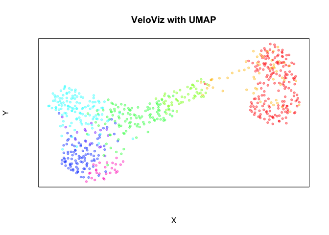
Now, use UMAP to embed the velocity informed graph constructed using VeloViz:
veloviz.nnGraph <- asNNGraph(veloviz.graph) #converts veloviz igraph object to a format that UMAP understands

set.seed(0)
emb.umapVelo <- uwot::umap(X = NULL, nn_method = veloviz.nnGraph, min_dist = 1)
rownames(emb.umapVelo) <- rownames(emb.veloviz)
plotEmbedding(emb.umapVelo, colors = cell.cols,
              main = 'VeloViz with UMAP', xlab = "X", ylab = "Y")
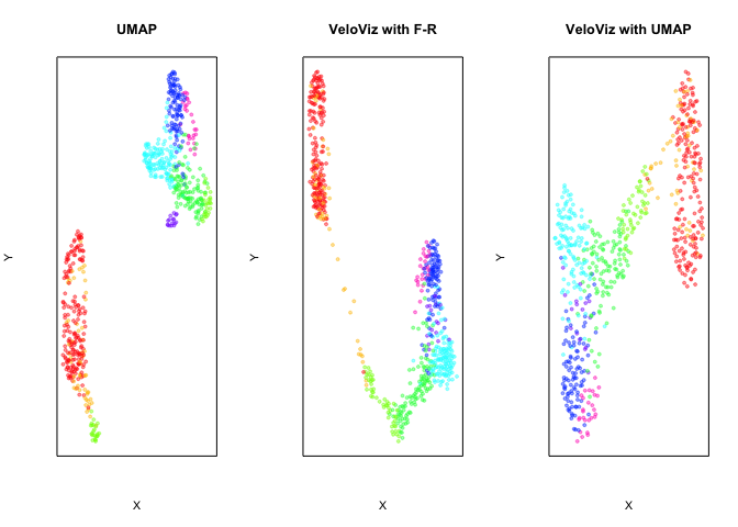
par(mfrow = c(1,3))

plotEmbedding(emb.umap, colors = cell.cols,
              main = 'UMAP', xlab = "X", ylab = "Y")
plotEmbedding(emb.veloviz, colors = cell.cols,
              main = 'VeloViz with F-R', xlab = "X", ylab = "Y")
plotEmbedding(emb.umapVelo, colors = cell.cols,
              main = 'VeloViz with UMAP', xlab = "X", ylab = "Y")
Let’s try it when there is a gap in the data. First, download the preprocessed example from Zenodo:
# get data
download.file("https://zenodo.org/record/4632471/files/pancreasWithGap.rda?download=1", destfile = "pancreasWithGap.rda", method = "curl")
load("pancreasWithGap.rda")

spliced = pancreasWithGap$spliced
unspliced = pancreasWithGap$unspliced
clusters = pancreasWithGap$clusters
pcs = pancreasWithGap$pcs

#choose colors based on clusters for plotting later
cell.cols = rainbow(8)[as.numeric(clusters)]
names(cell.cols) = names(clusters)
Compute velocity:
#cell distance in PC space
cell.dist = as.dist(1-cor(t(pcs))) # cell distance in PC space

vel = gene.relative.velocity.estimates(spliced,
                                       unspliced,
                                       kCells = 30,
                                       cell.dist = cell.dist,
                                       fit.quantile = 0.1)
#(or use precomputed velocity object) # vel = pancreasWithGap$vel
Embed using UMAP with PCs as inputs:
set.seed(0)
emb.umap <- uwot::umap(pcs, min_dist = 0.5)
rownames(emb.umap) <- rownames(pcs)

plotEmbedding(emb.umap, colors = cell.cols,
              main = 'UMAP', xlab = "X", ylab = "Y")
Now, build VeloViz graph:
curr <- vel$current
proj <- vel$projected

veloviz.graph <- buildVeloviz(
  curr = curr,
  proj = proj,
  normalize.depth = TRUE,
  use.ods.genes = TRUE,
  alpha = 0.05,
  pca = TRUE,
  nPCs = 20,
  center = TRUE,
  scale = TRUE,
  k = 20,
  similarity.threshold = 0,
  distance.weight = 1,
  distance.threshold = 0,
  weighted = TRUE,
  seed = 0,
  verbose = FALSE
)

emb.veloviz <- veloviz.graph$fdg_coords
plotEmbedding(emb.veloviz, colors = cell.cols,
              main = 'VeloViz with F-R', xlab = "X", ylab = "Y")
Now, use UMAP to embed the velocity informed graph constructed using VeloViz:
veloviz.nnGraph <- asNNGraph(veloviz.graph) #converts veloviz igraph object to a format that UMAP understands

set.seed(0)
emb.umapVelo <- uwot::umap(X = NULL, nn_method = veloviz.nnGraph, min_dist = 1)
rownames(emb.umapVelo) <- rownames(emb.veloviz)
plotEmbedding(emb.umapVelo, colors = cell.cols,
              main = 'VeloViz with UMAP', xlab = "X", ylab = "Y")
par(mfrow = c(1,3))

plotEmbedding(emb.umap, colors = cell.cols,
              main = 'UMAP', xlab = "X", ylab = "Y")
plotEmbedding(emb.veloviz, colors = cell.cols,
              main = 'VeloViz with F-R', xlab = "X", ylab = "Y")
plotEmbedding(emb.umapVelo, colors = cell.cols,
              main = 'VeloViz with UMAP', xlab = "X", ylab = "Y")
Other tutorials
Getting Started
scRNA-seq data preprocessing and visualization using VeloViz
MERFISH cell cycle visualization using VeloViz
Understanding VeloViz parameters
VeloViz with dynamic velocity estimates from scVelo