Standard figure of one gene in a compareSpatial() result

One figure for one gene of a compareSpatial() result: the gene's expression in the two samples at native resolution (the cells or spots, when the objects before rasterization are given), on the shared grid of pixels, the similarity class of every pixel, and the expression at matched pixels as a scatter plot labelled with the gene's statistics. The panels are lettered, one letter for each pair of maps, and the figure is ready to print, to save with ggplot2::ggsave() or to adjust with patchwork and ggplot2.

Usage

plotGene(
  result,
  gene,
  x,
  y = NULL,
  native = NULL,
  assay = NULL,
  nativeAssay = NULL,
  panels = c("native", "raster", "similarity", "scatter"),
  transform = c("none", "log1p"),
  sharedScale = TRUE,
  pointSize = NULL,
  nativeUnit = "cells",
  baseSize = 10,
  ...
)

Arguments

result: A compareSpatial() result.
gene: The gene (one row name of result) to plot.
x, y: The two rasterized SpatialExperiment objects that compareSpatial() compared, in the same order (or, as there, a list of the two as x with y = NULL). The sample names come from result.
native: Optional: a list of the two SpatialExperiment objects before rasterization, in the same order and in the same coordinate frame as the rasterized objects (for example aligned with STalign), for the native-resolution maps. Default NULL: no native maps.
assay: The assay of x and y to draw: a name or an index, or two (one per object). Default NULL: the assay that compareSpatial() used, from attr(result, "params").
nativeAssay: The assay of the native objects to draw, a name or an index, or two. Default NULL: the first assay.
panels: The panels to draw, in the order of Details; the figure keeps that order. Default: all. "native" needs native and is dropped without it; "similarity" is dropped when the classes cannot be computed (Details).
transform: The scale of the expression maps and of the scatter axes: "none" (default) or "log1p".
sharedScale: One colour scale for the two maps of a pair (default TRUE), or one per map (FALSE); see Details.
pointSize: The size of the points of the native maps (ggplot2's size). Default NULL: \(30 / \sqrt{n}\) for \(n\) cells or spots, between 0.1 and 1.5 at baseSize = 10 (about 0.85 for a thousand cells, 0.3 for ten thousand) and scaled with baseSize, so that the points of a dense tissue stay apart.
nativeUnit: What the points of the native maps are, for their subtitles: "cells" (default), "spots" for Visium, or two (one per sample).
baseSize: The base font size in points: the size of the axis titles, from which every other text, the legend keys and the points are scaled. Default 10, for a figure about 7 to 11 inches wide, depending on the tissue; 7 for a journal page of up to 180 mm (Details, Layout and size).
...: Passed to patchwork::wrap_plots(): ncol, nrow, design, widths, heights, guides.

Value

A patchwork object (a ggplot2 figure of the panels, lettered, titled with the gene and subtitled with the samples). Printing it draws the figure; ggplot2::ggsave() saves it.

Details

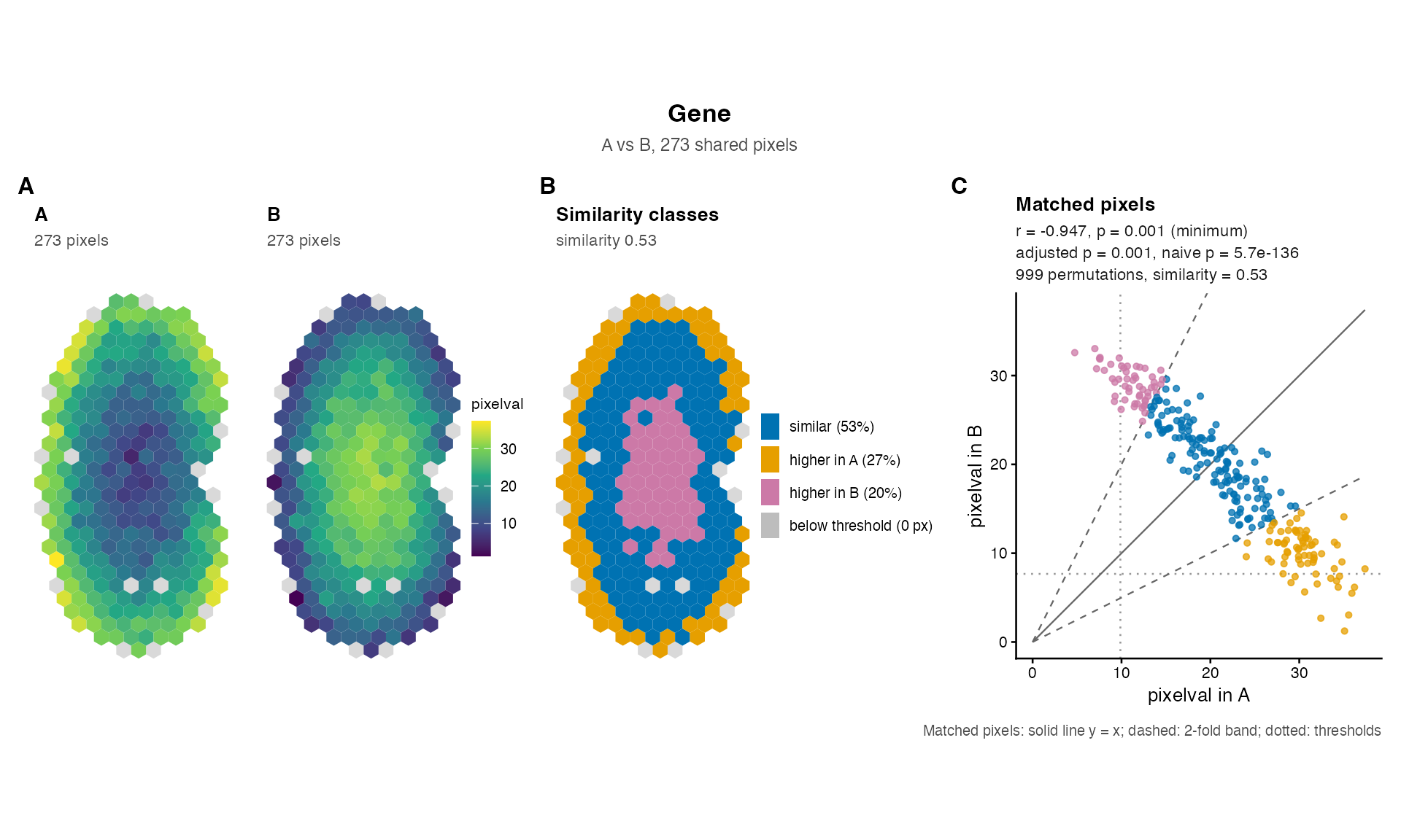
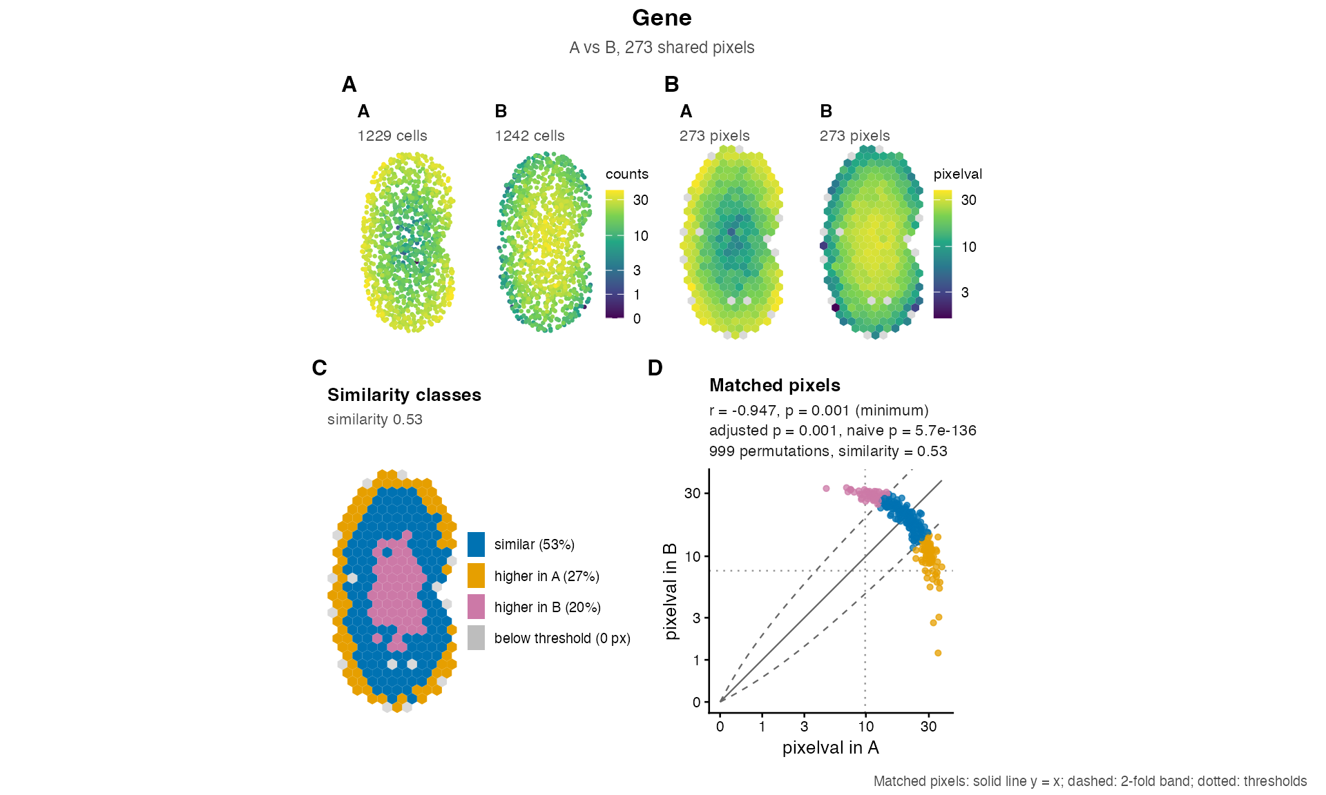
Panels. In this order, each map with the sample name as its title. The two maps of a pair share one letter (shown at the first map), so the full figure is lettered A to D and the figure without native maps A to C:

"native": Two maps of the cells or spots of native, coloured by the gene's expression in nativeAssay, each cell or spot a point (pointSize). Drawn only when native is given.
"raster": Two maps of the shared pixels (those the result used), coloured by the gene's expression in assay, the values the tests compared. The pixels are drawn with their geometry when the objects were rasterized with SEraster (colData() column geometry, which needs the sf package), otherwise as square tiles the size of the distance between neighbouring pixels. The pixels that one sample lacks (present in the other sample only, so not used by the tests) are drawn in light grey in every map, so that the outline of the tissue is complete and the maps are comparable.
"similarity": The shared pixels coloured by their class in the similarity test, recomputed from the data with the result's settings (foldChange, minPixels, and the gene's thresholds t1 and t2): similar (\(|\log_2(y/x)| \le\) foldChange), higher in the first sample, higher in the second sample, or below the threshold in both. The legend gives the share of each class among the pixels above the threshold, so that the share of similar pixels is the gene's percentSimilarity. Drawn when the result has the similarity columns and the gene's percentSimilarity is not NA: not for a gene with negative values (a fold change needs non-negative values), nor for a gene with fewer pixels above the threshold than minPixels allows; the scatter plot then says why.
"scatter": The expression at matched pixels, the first sample horizontally and the second vertically, on equal axes, coloured by the same classes (plain when they are not available), with the line \(y = x\) (solid), the fold-change band (dashed, slopes \(2^{foldChange}\) and \(2^{-foldChange}\)) and the thresholds (dotted); the figure's caption is the key to these lines. Its subtitle gives the gene's row of the result: correlationCoef (r), pValuePermute (p), pValuePermuteAdj (adjusted p), pValueNaive (naive p), the number of permutations and percentSimilarity (similarity), each to two significant digits; NA, with the reason from the result's message column, for a gene that was skipped or failed, whose status is then shown. p is marked (minimum) when it is \(1 / (nPermutations + 1)\), the smallest p-value the permutations can give, and a p-value of 0 is printed as < 2.2e-16.

A result without the correlation columns (tests = "similarity") gives a scatter subtitle with the similarity alone; a result without the similarity columns (tests = "correlation") has no similarity panel and a plain scatter plot.

Layout and size. Without native maps the panels are in one row; with them, the four expression maps are in the first row and the similarity map and the scatter plot, larger, in a second row. The maps keep the shape of the tissue, so the height of the figure sets the size of the panels and the tissue sets the width the figure needs: a wider canvas only adds blank space at the sides of a row. With the default baseSize = 10, ggplot2::ggsave(..., height = 6.5) suits two rows and height = 3.5 one row; a tissue that is taller than wide, like the kidneys of the examples, then fills width = 7 (two rows) or width = 8.5 (one row), and a square tissue about width = 10 or 11; a narrower canvas clips the statistics of the scatter plot. For a journal figure 180 mm wide, use baseSize = 7 with ggsave(..., width = 180, height = 110, units = "mm") for two rows or height = 60 for one row, and reduce the width for a taller tissue; for a single column of 90 mm, use baseSize = 6 and ncol = 2. Every text size follows baseSize, and patchwork's & operator rescales the whole figure: plotGene(...) & ggplot2::theme(text = ggplot2::element_text(size = 7)). The layout can be changed with the arguments of patchwork::wrap_plots() passed through ..., for example ncol = 2, and the figure with patchwork's operators, for example plotGene(...) + patchwork::plot_annotation(tag_levels = NULL) to remove the letters, or tag_levels = list(c("a", "", "b", "", "c", "d")) for lower-case letters (one entry per map, the second map of a pair blank).

Colour scales. The expression maps use the viridis palette. With sharedScale = TRUE the two native maps share one scale (one legend) and so do the two raster maps, so that the colours of the two samples are comparable. When the samples' values are on different scales (for example raw counts in one and normalized values in the other, or very different sequencing depths), sharedScale = FALSE gives every map its own scale and legend. transform = "log1p" draws the expression maps and the scatter axes on a \(\log(1 + v)\) scale, which spreads out the low values of counts; the classes and the statistics are unchanged, and the fold-change band is then curved. It needs values that are not negative.

Checks. The objects must be those that compareSpatial() compared: the function warns when they share another number of pixels than the result used (the classes are then recomputed on the pixels given), and when x and y appear to be swapped (the gene's thresholds t1 and t2 are those of the other sample). A named native list is put in the order of the result's samples when its names are the sample names, and taken in order, with a warning, when they are other names.

Examples

data(speKidney)
rast <- SEraster::rasterizeGeneExpression(speKidney, assay_name = "counts",
                                          resolution = 0.2, fun = "mean",
                                          square = FALSE)
ab <- compareSpatial(list(A = rast$A, B = rast$B), nPermutations = 999,
                     nThreads = 2)
#> compareSpatial: 1 gene on 273 shared pixels in 0.2 s (999 permutations in total, 2 threads)

# the pixels, the similarity classes and the scatter plot
plotGene(ab, "Gene", rast$A, rast$B)


# with the cells at native resolution, on a log1p colour scale
plotGene(ab, "Gene", rast$A, rast$B, native = speKidney[c("A", "B")],
         transform = "log1p")


# save it: for these kidneys, taller than wide, 8.5 x 3.5 inches without
# native maps and 7 x 6.5 with them; for a journal figure, baseSize = 7
if (FALSE) { # \dontrun{
ggplot2::ggsave("Gene.pdf", plotGene(ab, "Gene", rast$A, rast$B),
                width = 8.5, height = 3.5)
ggplot2::ggsave("Gene-cells.png",
                plotGene(ab, "Gene", rast$A, rast$B,
                         native = speKidney[c("A", "B")]),
                width = 7, height = 6.5, dpi = 300)
ggplot2::ggsave("Gene-140mm.pdf",
                plotGene(ab, "Gene", rast$A, rast$B, baseSize = 7),
                width = 140, height = 60, units = "mm")
} # }