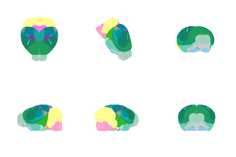
3D animation of the brain in R

Backstory
Over the years, I have come to accept that if I don’t put code online, I
will lose track of it and it will become lost in the ether. I wrote this
code awhile ago for a presentation, then proceeded to forget where I
saved the code, found the code again, and will now make a blog post for
the code as a tutorial for future me. So in this blog post, I will
explain to future me how to use data from the Allen Brain Atlas to
animate a 3D brain using the rgl package in R.
Getting the data
The Allen Brain Atlas offers downloads of 3D annotations of brain structure registered to their Mouse Common Coordinate Framework (CCF). Let’s get the brain structure annotations corresponding to the adult mouse brain CCF at 50um resolution.
## Download the 50um resolution 3D structural annotations
annot <- nat::read.nrrd('https://download.alleninstitute.org/informatics-archive/current-release/mouse_ccf/annotation/ccf_2017/annotation_50.nrrd')
## Registered S3 method overwritten by 'nat':
##   method             from
##   as.mesh3d.ashape3d rgl

## Warning in readBin(fc, what = dataTypes$what[i], n = dataLength, size =
## dataTypes$size[i], : 'signed = FALSE' is only valid for integers of sizes 1 and
## 2
dim(annot)
## [1] 264 160 228
Note that the data is in the form of a 264 by 160 by 228 matrix where each element is a structure ID. 0 corresponds to background.
## look at different small slices
annot[100:105,100:105,30]
##      [,1] [,2] [,3] [,4] [,5] [,6]
## [1,]  120  120  120  120  120    0
## [2,]  163  120  120  120  120  120
## [3,]  163  163  120  120  120  120
## [4,]  163  163  163  120  120  120
## [5,]  163  163  163  163  120  120
## [6,]  163  163  163  163  163  120
annot[100:105,100:105,50]
##      [,1] [,2] [,3] [,4] [,5] [,6]
## [1,]  783  783  583  583  583  952
## [2,]  579  579  579  783  703  703
## [3,]  672  672  672  579  579  579
## [4,]  672  672  672  672  672  579
## [5,]  672  672  672  672  672  672
## [6,]  672  672  672  672  672  672
We can obtain all the unique structure IDs and save them for future reference.
struc <- unique(as.numeric(annot))
head(struc)
## [1] 0 959 97 735 836 873
The Allen Brain Atlas also has a mapping of all these structure IDs to acronyms as well as colors used in their interactive atlas viewer and other info. We cam parse through to get the acronym and color information corresponding to structure IDs info in a table format.
url <- 'http://api.brain-map.org/api/v2/structure_graph_download/1.json'
library(magrittr)
raw_json <- url %>%
  httr::GET() %>%
  httr::content()
json_tb <- tidyjson::json_structure(raw_json)
head(json_tb)
## # A tbl_json: 6 x 10 tibble with a "JSON" attribute
##   ..JSON    document.id parent.id level index child.id seq    name  type  length
##   <chr>           <int> <chr>     <int> <int> <chr>    <list> <chr> <fct>  <int>
## 1 "true"              1 <NA>          0     1 1        <list> <NA>  logi…      1
## 2 "0"                 2 <NA>          0     1 1        <list> <NA>  numb…      1
## 3 "0"                 3 <NA>          0     1 1        <list> <NA>  numb…      1
## 4 "1"                 4 <NA>          0     1 1        <list> <NA>  numb…      1
## 5 "1"                 5 <NA>          0     1 1        <list> <NA>  numb…      1
## 6 "[{\"id\…           6 <NA>          0     1 1        <list> <NA>  array      1
map <- do.call(rbind, lapply(1:nrow(json_tb), function(i) {
  if(length(unlist(json_tb[i,]$..JSON[[1]])) > 6) {
    c(
      id = json_tb[i,]$..JSON[[1]]$id,
      atlas_id = json_tb[i,]$..JSON[[1]]$atlas_id,
      acronym = json_tb[i,]$..JSON[[1]]$acronym,
      col = paste0('#', json_tb[i,]$..JSON[[1]]$color_hex_triplet)
    )
  }
}))
## Warning in (function (..., deparse.level = 1) : number of columns of result is
## not a multiple of vector length (arg 23)
map <- map[map[,1] != "#",]
head(map)
##      id          atlas_id acronym        col
## [1,] "997"       "-1"     "root"         "#FFFFFF"
## [2,] "8"         "0"      "grey"         "#BFDAE3"
## [3,] "1009"      "691"    "fiber tracts" "#CCCCCC"
## [4,] "73"        "716"    "VS"           "#AAAAAA"
## [5,] "1024"      "693"    "grv"          "#AAAAAA"
## [6,] "304325711" "retina" "#7F2E7E"      "304325711"
For now, I will just focus on the mapping from structure IDs to colors.
allencol <- map[,4]
names(allencol) <- map[,1]
head(allencol)
##         997           8        1009          73        1024   304325711
##   "#FFFFFF"   "#BFDAE3"   "#CCCCCC"   "#AAAAAA"   "#AAAAAA" "304325711"
Plotting in 3D
In order to visualize these structures in 3D, I will get their 3D pixel
coordinates at 50um resolution from the annot 3D matrix and also keep
track of the structure’s corresponding colors using the allencol
mapping vector we just made.
Let’s try visualizing one structure first. We will pick structure ID 1009, which corresponds to the fiber tracts.
teststruc <- "1009"
strucpos <- which(annot == teststruc, arr.ind=TRUE)
struccol <- rep(allencol[as.character(teststruc)], nrow(strucpos))
strucposall <- data.frame(strucpos, col=struccol)
head(strucposall)
##   dim1 dim2 dim3     col
## 1  154  103   47 #CCCCCC
## 2  154  104   48 #CCCCCC
## 3  154  106   49 #CCCCCC
## 4  145   68   50 #CCCCCC
## 5  154  107   50 #CCCCCC
## 6  144   68   51 #CCCCCC
We can visualize this structures as points in 3D using rgl and make
some fun movies using the movie3d() and spin3d() functions in rgl.
library(rgl)
open3d()
view3d( theta = 90, phi = -90, fov = 0)
plot3d(strucpos[,1:3], col=struccol[4],
       size=1, axes = FALSE,  xlab='', ylab='', zlab='',
       aspect = dim(annot))
movie3d(spin3d(axis = c(1, 0, 0)), duration = 3, dir = getwd())
movie3d(spin3d(axis = c(0, 0, 1)), duration = 3, dir = getwd())
movie3d(spin3d(axis = c(0, 1, 0)), duration = 15, dir = getwd())

Now we can do loop through and do this for all the structures.
## ignore background struc[1]
strucposall <- do.call(rbind, lapply(struc[-1], function(teststruc) {
  strucpos <- which(annot == teststruc, arr.ind=TRUE)
  struccol <- rep(allencol[as.character(teststruc)], nrow(strucpos))
  data.frame(strucpos, col=struccol)
}))
head(strucposall)
##   dim1 dim2 dim3     col
## 1  156   67   12 #019399
## 2  157   67   12 #019399
## 3  158   67   12 #019399
## 4  159   67   12 #019399
## 5  160   67   12 #019399
## 6  161   67   12 #019399
open3d()
view3d( theta = 90, phi = -90, fov = 0)
plot3d(strucposall[,1:3], col=strucposall[,4],
       size=1, axes = FALSE,  xlab='', ylab='', zlab='',
       aspect = dim(annot))
movie3d(spin3d(axis = c(1, 0, 0)), duration = 3, dir = getwd())
movie3d(spin3d(axis = c(0, 0, 1)), duration = 3, dir = getwd())
movie3d(spin3d(axis = c(0, 1, 0)), duration = 15, dir = getwd())

We can even focus on a specific coronal slice cutting from 150 pixels to 180 pixels (multiple by 50um to mentally convert back to microns).
vi <- strucposall[,1] > 150 & strucposall[,1] < 180
view3d( theta = 90, phi = -90, fov = 0)
plot3d(strucposall[vi,1:3], col=strucposall[vi,4],
       size=1, axes = FALSE,  xlab='', ylab='', zlab='',
       aspect = dim(annot),
       xlim = c(0, dim(annot)[1]))
movie3d(spin3d(axis = c(1, 0, 0)), duration = 3, dir = getwd())
movie3d(spin3d(axis = c(0, 0, 1)), duration = 3, dir = getwd())
movie3d(spin3d(axis = c(0, 1, 0)), duration = 15, dir = getwd())

Try it out for yourself
- Visualize a different brain structure.
- Visualize a different coronal slice.
- What if we use a higher resolution structural annotation to begin with?
- How do we integrate with meshes instead of discrete points?
Additional resources
Recent Posts
- The Mentorship Index on 01 March 2026
- Vibe coding with SEraster and STcompare to compare spatial transcriptomics technologies on 22 February 2026
- RNA velocity in situ infers gene expression dynamics using spatial transcriptomics data on 13 October 2025
- Analyzing ICE Arrest Data - Part 2 on 27 September 2025
- Analyzing ICE Detention Data from 2021 to 2025 on 10 July 2025