
STcompare to identify spatially sexually dimorphic genes in mouse kidneys
We recently developed an R package to perform spatial differential expression analysis called STcompare. The details of the method can be found in our paper in Oxford Bioinformatics. In our paper, we highlight how, given two spatial transcriptomics datasets to be compared such as in a healthy vs diseased setting, some genes may not be considered globally differentially expressed and yet exhibit distinct spatial patterns. STcompare enables the identification of such genes.
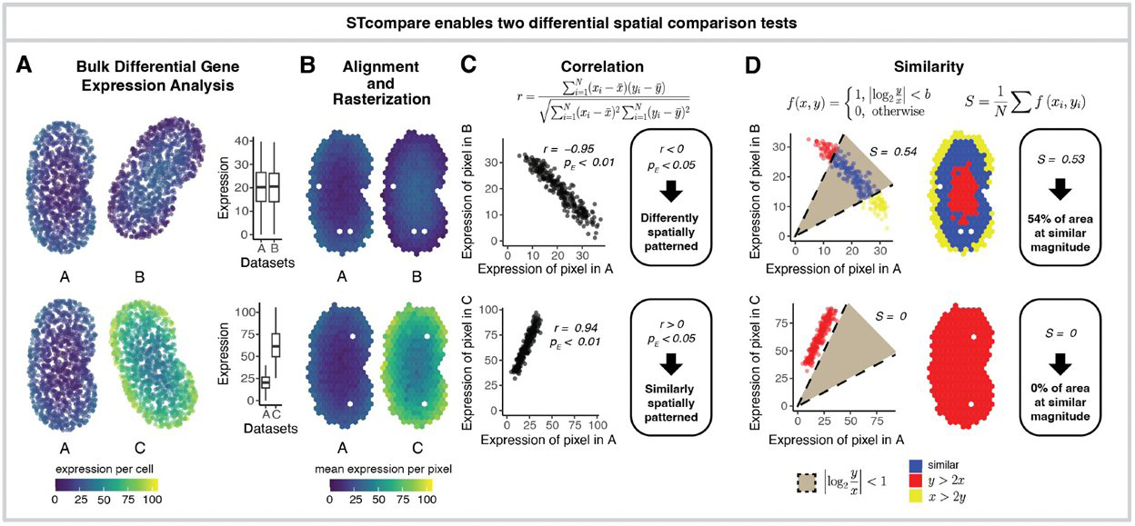
In this tutorial, I will use STcompare to compare spatial transcriptomic data of a female and male mouse kidney to identify spatially sexually dimorphic genes.
Setting up
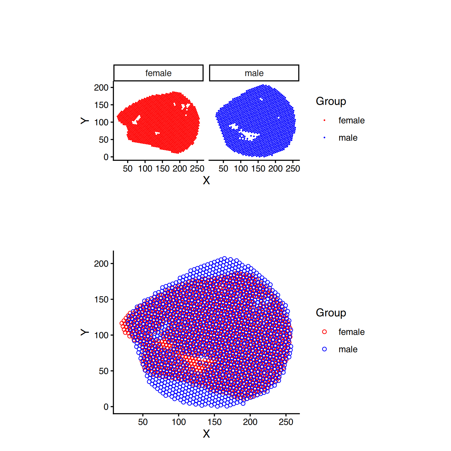
I downloaded Visium spatial transcriptomics datasets for a sham/normal female mouse kidney from Dixon et al as well as a sham/normal male mouse kidney from Xuanyuan et al. Because STcompare requires tissues to be pre-aligned into a common coordinate space, I performed a manual affine alignment (that is not great but enough to let us test out STcompare).
You can download my processed version of this data to follow along this tutorial:
Initial vibe coding attempt
I initially tried to use vibe coding to do this analysis (but ultimately found it easier to just copy and modify from the STcompare vignettes).
I cloned the STcompare Github repo into my working directory so that my AI agent could read the code and also the tutorials. STcompare already provides a vignette for analyzing Visium data for acute kidney injury so I figured it would be straight-forward to simply follow that tutorial but apply it to our new data. In my prompt, I described the data, directory structure, what I would like the agent to code, how the output should be organized.
Prompt:
The
data/folder contains two Visium spatial transcriptomics datasets calledvisium_female1_kidney_shamcontrol.csv.gzandvisium_male1_kidney_shamcontrol.csv.gzwhere each row is spot, the columns correspond to the spot ID, the X and Y positions of the affine-aligned spots, and gene names.
The
STcompare/folder contains an R package for spatial differential expression analysis.
Install the package and follow the Acute Kidney Injury (10x Visium) Application tutorial in the vignettes/ folder to write an R script called
female_male_kidney_STcompare.Rthat reads in the two Visium spatial transcriptomics datasets and evaluates all genes for spatial differential expression. Note that the two Visium spatial transcriptomics datasets used here have already been affine-aligned.
Save STcompare visualizations in the
results/folder. Save all numeric results as a csv file. Save all p-values and do not filter out insignificant hits.
The resulting code was quite a bit more complex than what I thought was necessary. The AI seems to have reengineered a lot of functions rather than just running them as is from the tutorial.
#!/usr/bin/env Rscript
#
# female_male_kidney_STcompare.R
#
# Compare affine-aligned female and male Visium kidney sham-control sections
# with STcompare, following the Acute Kidney Injury (10x Visium) Application
# vignette. Alignment is skipped because the two CSVs are already affine-aligned.
# Analysis is restricted to genes that are spatially variable (SVGs) in both
# samples. STcompare p-values are written without dropping insignificant hits.

## Paths #######################################################################

args <- commandArgs(trailingOnly = FALSE)
file_arg <- grep("^--file=", args, value = TRUE)
if (length(file_arg) == 1) {
  root <- dirname(normalizePath(sub("^--file=", "", file_arg)))
} else {
  root <- getwd()
}

data_dir <- file.path(root, "data")
results_dir <- file.path(root, "results")
gene_plot_dir <- file.path(results_dir, "gene_plots")
dir.create(results_dir, showWarnings = FALSE, recursive = TRUE)
dir.create(gene_plot_dir, showWarnings = FALSE, recursive = TRUE)

female_path <- file.path(data_dir, "visium_female1_kidney_shamcontrol.csv.gz")
male_path <- file.path(data_dir, "visium_male1_kidney_shamcontrol.csv.gz")

log_msg <- function(...) {
  msg <- paste0(format(Sys.time(), "%Y-%m-%d %H:%M:%S"), "  ", paste(..., collapse = " "))
  cat(msg, "\n", sep = "")
  flush.console()
}

save_plot <- function(plot, name, width = 8, height = 6) {
  ggplot2::ggsave(
    filename = file.path(results_dir, paste0(name, ".pdf")),
    plot = plot, width = width, height = height, units = "in"
  )
  ggplot2::ggsave(
    filename = file.path(results_dir, paste0(name, ".png")),
    plot = plot, width = width, height = height, units = "in", dpi = 150
  )
}

## Install / load packages #####################################################

stcompare_src <- file.path(root, "STcompare")
if (!requireNamespace("STcompare", quietly = TRUE)) {
  if (!requireNamespace("remotes", quietly = TRUE)) {
    install.packages("remotes", repos = "https://cloud.r-project.org")
  }
  remotes::install_local(
    stcompare_src,
    upgrade = "never",
    dependencies = FALSE,
    build_vignettes = FALSE
  )
}

suppressPackageStartupMessages({
  library(STcompare)
  library(SpatialExperiment)
  library(SEraster)
  library(SummarizedExperiment)
  library(Matrix)
  library(ggplot2)
  library(dplyr)
  library(patchwork)
  library(BiocParallel)
  library(MERINGUE)
})

n_threads <- parallel::detectCores(logical = FALSE)
if (is.na(n_threads) || n_threads < 1) {
  n_threads <- 8L
}
# Avoid BLAS/OpenMP fighting BiocParallel workers
Sys.setenv(OMP_NUM_THREADS = "1", MKL_NUM_THREADS = "1", OPENBLAS_NUM_THREADS = "1")

log_msg("Using", n_threads, "threads")

## Load Visium CSVs ############################################################
# Each row is a spot. After the barcode rownames, columns are affine-aligned
# X/Y coordinates followed by gene counts. Files may be plain CSV despite the
# .gz suffix.

read_visium_csv <- function(path) {
  con <- file(path, "rb")
  magic <- readBin(con, what = "raw", n = 2)
  close(con)
  is_gz <- length(magic) >= 2 && identical(as.integer(magic), c(0x1f, 0x8b))
  if (is_gz) {
    read.csv(gzfile(path), row.names = 1, check.names = FALSE)
  } else {
    read.csv(path, row.names = 1, check.names = FALSE)
  }
}

log_msg("Reading female:", female_path)
female_df <- read_visium_csv(female_path)
log_msg("Reading male:", male_path)
male_df <- read_visium_csv(male_path)

stopifnot(all(c("X", "Y") %in% colnames(female_df)))
stopifnot(all(c("X", "Y") %in% colnames(male_df)))

genes_female <- setdiff(colnames(female_df), c("X", "Y"))
genes_male <- setdiff(colnames(male_df), c("X", "Y"))
shared_genes <- intersect(genes_female, genes_male)
log_msg(
  "Spots female/male:", nrow(female_df), "/", nrow(male_df),
  "; genes female/male/shared:",
  length(genes_female), "/", length(genes_male), "/", length(shared_genes)
)

csv_to_spe <- function(df, genes, sample_name) {
  pos <- as.matrix(df[, c("X", "Y"), drop = FALSE])
  colnames(pos) <- c("x", "y")
  rownames(pos) <- rownames(df)
  counts <- t(as.matrix(df[, genes, drop = FALSE]))
  counts <- as(counts, "dgCMatrix")
  colnames(counts) <- rownames(df)
  SpatialExperiment::SpatialExperiment(
    assays = list(counts = counts),
    spatialCoords = pos
  )
}

female_spe <- csv_to_spe(female_df, shared_genes, "female")
male_spe <- csv_to_spe(male_df, shared_genes, "male")
rm(female_df, male_df)
gc(verbose = FALSE)

## Aligned positions (already affine-aligned) ##################################

female_pos <- as.data.frame(SpatialExperiment::spatialCoords(female_spe))
male_pos <- as.data.frame(SpatialExperiment::spatialCoords(male_spe))
female_pos$group <- "Female"
male_pos$group <- "Male"
pos_df <- rbind(female_pos, male_pos)

pos_plot <- ggplot(pos_df, aes(x = x, y = y, color = group)) +
  geom_point(size = 0.5, alpha = 0.7) +
  scale_color_manual(values = c("Female" = "#1f77b4", "Male" = "#d62728")) +
  coord_fixed() +
  labs(
    x = "x", y = "y", color = "Sample",
    title = "Affine-aligned female and male kidney Visium spots"
  ) +
  theme_classic()
save_plot(pos_plot, "aligned_spot_positions", width = 8, height = 6)
log_msg("Saved aligned spot position plot")

## Rasterize to a shared hexagonal pixel grid ##################################
# Same settings as the AKI Visium vignette: hexagonal pixels, sum aggregation,
# resolution = 5. Rasterization creates one-to-one pixels for STcompare.

# Vignette uses resolution = 5; 20 yields coarser pixels and a faster run.
# Neighbor distance for Moran's I is 2x resolution, as in the vignette.
resolution <- 20
filter_dist <- 2 * resolution

log_msg("Rasterizing gene expression at resolution", resolution)
spe_list <- list(female = female_spe, male = male_spe)
rast <- SEraster::rasterizeGeneExpression(
  spe_list,
  resolution = resolution,
  fun = "sum",
  square = FALSE,
  assay_name = "counts"
)

# SEraster stores rasterized values in the first assay (typically "pixelval")
keep_nonzero_pixels <- function(se) {
  se[, Matrix::colSums(SummarizedExperiment::assay(se, 1)) > 0]
}
rast$female <- keep_nonzero_pixels(rast$female)
rast$male <- keep_nonzero_pixels(rast$male)

# CPM normalization after rasterization, as in the vignette
SummarizedExperiment::assay(rast$female, "CPM") <-
  Matrix::t(Matrix::t(SummarizedExperiment::assay(rast$female, 1)) /
              Matrix::colSums(SummarizedExperiment::assay(rast$female, 1))) * 1e6
SummarizedExperiment::assay(rast$male, "CPM") <-
  Matrix::t(Matrix::t(SummarizedExperiment::assay(rast$male, 1)) /
              Matrix::colSums(SummarizedExperiment::assay(rast$male, 1))) * 1e6

shared_pixels <- intersect(
  rownames(SpatialExperiment::spatialCoords(rast$female)),
  rownames(SpatialExperiment::spatialCoords(rast$male))
)
log_msg(
  "Raster pixels female/male/shared:",
  ncol(rast$female), "/", ncol(rast$male), "/", length(shared_pixels)
)

p_rast_f <- SEraster::plotRaster(
  rast$female, assay_name = "CPM", name = "total expression"
) + ggplot2::ggtitle("Female (rasterized CPM)")
p_rast_m <- SEraster::plotRaster(
  rast$male, assay_name = "CPM", name = "total expression"
) + ggplot2::ggtitle("Male (rasterized CPM)")
save_plot(p_rast_f + p_rast_m, "raster_total_expression", width = 12, height = 5)
log_msg("Saved rasterized total expression plot")

## Identify SVGs with Moran's I ################################################
# Same approach as the AKI Visium vignette: neighbor graph at 2x the raster
# resolution, Moran's I on the CPM assay, and SVGs defined as p.adj == 0.
# STcompare is then restricted to genes that are SVGs in both samples.

moransI <- function(SE_temp, filterDist, assayName = "CPM", plot_path = NULL) {
  coords <- SpatialExperiment::spatialCoords(SE_temp)
  w <- MERINGUE::getSpatialNeighbors(coords, filterDist = filterDist)
  if (!is.null(plot_path)) {
    grDevices::pdf(plot_path, width = 6, height = 6)
    par(mfrow = c(1, 1))
    MERINGUE::plotNetwork(coords, w)
    grDevices::dev.off()
  }
  MERINGUE::getSpatialPatterns(SummarizedExperiment::assays(SE_temp)[[assayName]], w)
}

log_msg("Computing Moran's I for female (filterDist =", filter_dist, ")")
moransI_female <- moransI(
  rast$female,
  filterDist = filter_dist,
  assayName = "CPM",
  plot_path = file.path(results_dir, "spatial_neighbors_female.pdf")
)
log_msg("Computing Moran's I for male (filterDist =", filter_dist, ")")
moransI_male <- moransI(
  rast$male,
  filterDist = filter_dist,
  assayName = "CPM",
  plot_path = file.path(results_dir, "spatial_neighbors_male.pdf")
)

utils::write.csv(
  cbind(gene = rownames(moransI_female), moransI_female),
  file.path(results_dir, "moransI_female.csv"),
  row.names = FALSE
)
utils::write.csv(
  cbind(gene = rownames(moransI_male), moransI_male),
  file.path(results_dir, "moransI_male.csv"),
  row.names = FALSE
)

svg_female <- moransI_female %>% dplyr::filter(p.adj == 0) %>% rownames()
svg_male <- moransI_male %>% dplyr::filter(p.adj == 0) %>% rownames()
svg_int <- intersect(svg_female, svg_male)
log_msg(
  "SVGs female/male/both:",
  length(svg_female), "/", length(svg_male), "/", length(svg_int)
)

# MERINGUE makes gene names syntactically valid; match raster rownames to that.
rownames(rast$female) <- make.names(rownames(rast$female), unique = TRUE)
rownames(rast$male) <- make.names(rownames(rast$male), unique = TRUE)
stopifnot(identical(rownames(rast$female), rownames(rast$male)))
if (length(setdiff(svg_int, rownames(rast$female))) > 0) {
  stop("SVG names do not match rasterized gene names after make.names().")
}
if (length(svg_int) == 0) {
  stop("No genes were spatially variable in both samples.")
}

genes_chosen <- svg_int
input <- list(
  female = rast$female[genes_chosen, ],
  male = rast$male[genes_chosen, ]
)

## Spatial fold-change similarity ##############################################

log_msg("Running spatialSimilarity on SVGs shared by both samples")
ss <- STcompare::spatialSimilarity(
  input = input,
  foldChange = 1,
  assayName = "CPM",
  t1 = NULL,
  t2 = NULL
)
log_msg("Finished spatialSimilarity")

## Spatial correlation with iterative permutations #############################
# Matches the vignette:
#   delta sequence includes 0.01 and 0.05 plus 0.1-0.9
#   nPermutations = c(100, 1000)
# Genes are checkpointed so a long run can be resumed.

delta_seq <- c(0.01, 0.05, seq(0.1, 0.9, 0.1))
n_permutations <- c(100, 1000)
alpha <- 0.05

run_spatial_correlation_genes <- function(genes,
                                          source,
                                          target,
                                          shared_pixels,
                                          pos,
                                          n_permutations,
                                          delta_seq,
                                          n_threads,
                                          seed,
                                          checkpoint_path) {
  if (file.exists(checkpoint_path)) {
    results <- readRDS(checkpoint_path)
    log_msg("Resuming", basename(checkpoint_path), "with", nrow(results), "genes")
  } else {
    results <- NULL
  }
  done <- if (is.null(results)) {
    character(0)
  } else {
    rownames(results)[
      !is.na(results$pValuePermuteX) & !is.na(results$pValuePermuteY)
    ]
  }
  if (!is.null(results) && length(done) < nrow(results)) {
    log_msg(
      "Retrying", nrow(results) - length(done),
      "checkpointed genes that have missing permutation p-values"
    )
    results <- if (length(done) == 0) NULL else results[done, , drop = FALSE]
  }
  todo <- setdiff(genes, done)
  log_msg(
    "nPermutations =", n_permutations,
    "; genes remaining:", length(todo), "/", length(genes)
  )

  if (length(todo) == 0) {
    return(results[genes, , drop = FALSE])
  }

  empty_result <- function(gene) {
    out <- data.frame(
      correlationCoef = NA_real_,
      pValueNaive = NA_real_,
      pValuePermuteX = NA_real_,
      pValuePermuteY = NA_real_,
      deltaStarMedianX = NA_real_,
      deltaStarMedianY = NA_real_,
      deltaStarX = I(list(NA)),
      deltaStarY = I(list(NA)),
      nullCorrelationsX = I(list(NA)),
      nullCorrelationsY = I(list(NA))
    )
    rownames(out) <- gene
    out
  }

  # Parallelize over genes with SOCK workers. Do not use MulticoreParam:
  # reusing its forked reducer causes
  # "wrong args for environment subassignment" on macOS.
  n_workers <- min(n_threads, length(todo))
  bp <- BiocParallel::SnowParam(
    workers = n_workers,
    type = "SOCK",
    stop.on.error = FALSE,
    progressbar = FALSE
  )
  BiocParallel::bpstart(bp)
  on.exit({
    if (BiocParallel::bpisup(bp)) {
      BiocParallel::bpstop(bp)
    }
  }, add = TRUE)

  batch_size <- max(n_workers, 10L)
  batch_starts <- seq(1L, length(todo), by = batch_size)
  for (b in seq_along(batch_starts)) {
    i0 <- batch_starts[b]
    i1 <- min(i0 + batch_size - 1L, length(todo))
    batch_genes <- todo[i0:i1]
    log_msg(
      sprintf(
        "nPermutations=%s | genes %d-%d/%d",
        n_permutations, i0, i1, length(todo)
      )
    )

    Xmat <- as.matrix(
      SummarizedExperiment::assay(source, "CPM")[batch_genes, shared_pixels, drop = FALSE]
    )
    Ymat <- as.matrix(
      SummarizedExperiment::assay(target, "CPM")[batch_genes, shared_pixels, drop = FALSE]
    )

    batch_res <- BiocParallel::bplapply(batch_genes, function(gene) {
      out <- STcompare::spatialCorrelation(
        as.numeric(Xmat[gene, ]),
        as.numeric(Ymat[gene, ]),
        pos,
        nPermutations = n_permutations,
        deltaX = delta_seq,
        deltaY = delta_seq,
        nThreads = 1L,
        BPPARAM = BiocParallel::SerialParam(),
        seed = seed
      )
      rownames(out) <- gene
      out
    }, BPPARAM = bp)

    for (j in seq_along(batch_genes)) {
      gene <- batch_genes[j]
      x <- batch_res[[j]]
      if (inherits(x, "try-error") || !is.data.frame(x)) {
        log_msg("Correlation failed for", gene, ":", paste(as.character(x), collapse = " "))
        x <- empty_result(gene)
      }
      results <- rbind(results, x)
    }
    saveRDS(results, checkpoint_path)
  }

  results[genes, , drop = FALSE]
}

pos_shared <- SpatialExperiment::spatialCoords(rast$female)[shared_pixels, ]
checkpoint_100 <- file.path(results_dir, "spatial_correlation_nperm100.rds")
checkpoint_1000 <- file.path(results_dir, "spatial_correlation_nperm1000.rds")

log_msg("Running spatial correlation (iterative permutations)")
corr_100 <- run_spatial_correlation_genes(
  genes = genes_chosen,
  source = rast$female,
  target = rast$male,
  shared_pixels = shared_pixels,
  pos = pos_shared,
  n_permutations = n_permutations[1],
  delta_seq = delta_seq,
  n_threads = n_threads,
  seed = 0,
  checkpoint_path = checkpoint_100
)

# Rerun genes that remain potentially significant at the next permutation count,
# using the same screening rule as spatialCorrelationGeneExpIterPermutations:
# both empirical p-values below (alpha / nPermutations) * 100.
screen_t <- (alpha / n_permutations[1]) * 100
genes_rerun <- rownames(corr_100)[
  which(
    !is.na(corr_100$pValuePermuteX) &
      !is.na(corr_100$pValuePermuteY) &
      corr_100$pValuePermuteX < screen_t &
      corr_100$pValuePermuteY < screen_t
  )
]
log_msg("Genes advancing to", n_permutations[2], "permutations:", length(genes_rerun))

if (length(genes_rerun) > 0) {
  corr_1000 <- run_spatial_correlation_genes(
    genes = genes_rerun,
    source = rast$female,
    target = rast$male,
    shared_pixels = shared_pixels,
    pos = pos_shared,
    n_permutations = n_permutations[2],
    delta_seq = delta_seq,
    n_threads = n_threads,
    seed = 0,
    checkpoint_path = checkpoint_1000
  )
  corr_100[rownames(corr_1000), colnames(corr_1000)] <- corr_1000
}

kidney_correlation <- corr_100
kidney_correlation$pValuePermuteX_raw <- kidney_correlation$pValuePermuteX
kidney_correlation$pValuePermuteY_raw <- kidney_correlation$pValuePermuteY
kidney_correlation$pValuePermuteX <- stats::p.adjust(
  kidney_correlation$pValuePermuteX_raw, method = "BH"
)
kidney_correlation$pValuePermuteY <- stats::p.adjust(
  kidney_correlation$pValuePermuteY_raw, method = "BH"
)
kidney_correlation$nPermutations <- vapply(
  kidney_correlation$deltaStarX,
  function(x) {
    x <- unlist(x)
    if (is.null(x) || length(x) == 0 || all(is.na(x))) {
      NA_integer_
    } else {
      as.integer(length(x))
    }
  },
  integer(1)
)
saveRDS(kidney_correlation, file.path(results_dir, "spatial_correlation.rds"))
log_msg("Finished spatial correlation for", nrow(kidney_correlation), "genes")

## Numeric results table (SVGs in both samples, no significance filter) ########

sim_tbl <- ss$similarityTable
sim_numeric <- data.frame(
  gene = sim_tbl$gene,
  percentSimilarity = sim_tbl$percentSimilarity,
  percentDissimilarityX = sim_tbl$percentDissimilarityX,
  percentDissimilarityY = sim_tbl$percentDissimilarityY,
  numPixelInThresh = sim_tbl$numPixelInThresh,
  numPixelOutThresh = sim_tbl$numPixelOutThresh,
  t1 = sim_tbl$t1,
  t2 = sim_tbl$t2,
  stringsAsFactors = FALSE
)

corr_numeric <- data.frame(
  gene = rownames(kidney_correlation),
  correlationCoef = kidney_correlation$correlationCoef,
  pValueNaive = kidney_correlation$pValueNaive,
  pValuePermuteX_raw = kidney_correlation$pValuePermuteX_raw,
  pValuePermuteY_raw = kidney_correlation$pValuePermuteY_raw,
  pValuePermuteX = kidney_correlation$pValuePermuteX,
  pValuePermuteY = kidney_correlation$pValuePermuteY,
  pValueEmpirical = pmax(
    kidney_correlation$pValuePermuteX,
    kidney_correlation$pValuePermuteY,
    na.rm = FALSE
  ),
  deltaStarMedianX = kidney_correlation$deltaStarMedianX,
  deltaStarMedianY = kidney_correlation$deltaStarMedianY,
  nPermutations = kidney_correlation$nPermutations,
  stringsAsFactors = FALSE
)

moran_female <- data.frame(
  gene = rownames(moransI_female),
  moranI_female = moransI_female$observed,
  moranPadj_female = moransI_female$p.adj,
  stringsAsFactors = FALSE
)
moran_male <- data.frame(
  gene = rownames(moransI_male),
  moranI_male = moransI_male$observed,
  moranPadj_male = moransI_male$p.adj,
  stringsAsFactors = FALSE
)

results_tbl <- data.frame(
  gene = genes_chosen,
  svg_female = TRUE,
  svg_male = TRUE,
  stringsAsFactors = FALSE
)
results_tbl <- results_tbl %>%
  dplyr::left_join(moran_female, by = "gene") %>%
  dplyr::left_join(moran_male, by = "gene") %>%
  dplyr::left_join(corr_numeric, by = "gene") %>%
  dplyr::left_join(sim_numeric, by = "gene") %>%
  dplyr::arrange(pValueEmpirical, dplyr::desc(abs(correlationCoef)))

csv_path <- file.path(results_dir, "female_male_kidney_STcompare_results.csv")
utils::write.csv(results_tbl, csv_path, row.names = FALSE)
log_msg("Wrote numeric results:", csv_path, "rows:", nrow(results_tbl))

## Summary visualizations ######################################################

sig_pos <- kidney_correlation %>%
  dplyr::filter(
    !is.na(pValuePermuteX), !is.na(pValuePermuteY),
    pValuePermuteX < 0.05, pValuePermuteY < 0.05,
    correlationCoef > 0
  ) %>%
  rownames()
sig_neg <- kidney_correlation %>%
  dplyr::filter(
    !is.na(pValuePermuteX), !is.na(pValuePermuteY),
    pValuePermuteX < 0.05, pValuePermuteY < 0.05,
    correlationCoef < 0
  ) %>%
  rownames()
log_msg("Significant positive/negative genes:", length(sig_pos), "/", length(sig_neg))

violin_df <- kidney_correlation %>%
  dplyr::mutate(
    gene = rownames(kidney_correlation),
    Sig = dplyr::case_when(
      gene %in% sig_pos ~ "SigPos",
      gene %in% sig_neg ~ "SigNeg",
      .default = "NotSig"
    )
  )
fig_violin <- ggplot2::ggplot(
  violin_df, ggplot2::aes(x = Sig, y = correlationCoef, color = Sig)
) +
  ggplot2::geom_violin() +
  ggplot2::geom_jitter(width = 0.2, alpha = 0.08) +
  ggplot2::ylim(-1, 1) +
  ggplot2::scale_color_manual(
    values = c("SigPos" = "green", "SigNeg" = "blue", "NotSig" = "grey")
  ) +
  ggplot2::theme_classic() +
  ggplot2::labs(
    x = "Significance",
    y = "Correlation coefficient",
    title = "Spatial correlation for SVGs in both samples (no significance filter on saved results)"
  )
save_plot(fig_violin, "correlation_coefficient_violin", width = 8, height = 6)

volcano_df <- violin_df %>%
  dplyr::mutate(
    pValueEmpirical = dplyr::case_when(
      pValuePermuteY > pValuePermuteX ~ pValuePermuteY,
      .default = pValuePermuteX
    ),
    pValueEmpiricalPlot = dplyr::if_else(
      is.na(pValueEmpirical) | pValueEmpirical == 0, 1e-4, pValueEmpirical
    )
  )
fig_volcano <- ggplot2::ggplot(
  volcano_df,
  ggplot2::aes(x = correlationCoef, y = -log10(pValueEmpiricalPlot), color = Sig)
) +
  ggplot2::geom_point(alpha = 0.35, size = 1.2) +
  ggplot2::geom_hline(yintercept = -log10(0.05), linetype = "dashed") +
  ggplot2::scale_color_manual(
    values = c("SigPos" = "green", "SigNeg" = "blue", "NotSig" = "grey")
  ) +
  ggplot2::theme_classic() +
  ggplot2::labs(
    x = "Correlation coefficient, r",
    y = "-log10(empirical p-value)",
    title = "Spatial correlation vs empirical p-value for SVGs in both samples"
  )
save_plot(fig_volcano, "correlation_vs_pvalue", width = 8, height = 6)

sim_corr <- data.frame(
  gene = rownames(kidney_correlation),
  correlation = kidney_correlation$correlationCoef,
  similar = ss$similarityTable$percentSimilarity[match(
    rownames(kidney_correlation), ss$similarityTable$gene
  )],
  percentDissimilarityX = ss$similarityTable$percentDissimilarityX[match(
    rownames(kidney_correlation), ss$similarityTable$gene
  )],
  percentDissimilarityY = ss$similarityTable$percentDissimilarityY[match(
    rownames(kidney_correlation), ss$similarityTable$gene
  )],
  stringsAsFactors = FALSE
) %>%
  dplyr::mutate(
    Sig = dplyr::case_when(
      gene %in% sig_pos ~ "SigPos",
      gene %in% sig_neg ~ "SigNeg",
      .default = "NotSig"
    )
  )

fig_sim_corr <- ggplot2::ggplot(
  sim_corr,
  ggplot2::aes(x = correlation, y = similar, color = Sig)
) +
  ggplot2::geom_point(alpha = 0.35, size = 1.2) +
  ggplot2::xlim(-1, 1) +
  ggplot2::ylim(0, 1) +
  ggplot2::scale_color_manual(
    values = c("SigPos" = "green", "SigNeg" = "blue", "NotSig" = "grey")
  ) +
  ggplot2::theme_classic() +
  ggplot2::labs(
    x = "Correlation",
    y = "Similarity",
    title = "Correlation vs fold-change similarity for SVGs in both samples"
  )
save_plot(fig_sim_corr, "correlation_vs_similarity", width = 8, height = 6)

## Example gene visualizations #################################################

pick_example_genes <- function(sim_corr, sig_pos, sig_neg) {
  gene1 <- sim_corr %>%
    dplyr::filter(gene %in% sig_pos) %>%
    dplyr::arrange(similar, dplyr::desc(correlation)) %>%
    dplyr::pull(gene) %>%
    head(1)
  if (length(gene1) == 0) {
    gene1 <- sim_corr %>%
      dplyr::arrange(dplyr::desc(correlation)) %>%
      dplyr::pull(gene) %>%
      head(1)
  }
  gene2 <- sim_corr %>%
    dplyr::filter(gene %in% sig_neg) %>%
    dplyr::mutate(diff = abs(percentDissimilarityX - percentDissimilarityY)) %>%
    dplyr::arrange(diff) %>%
    dplyr::pull(gene) %>%
    head(1)
  if (length(gene2) == 0) {
    gene2 <- sim_corr %>%
      dplyr::arrange(correlation) %>%
      dplyr::pull(gene) %>%
      head(1)
  }
  unique(c(gene1, gene2))
}

example_genes <- pick_example_genes(sim_corr, sig_pos, sig_neg)
# Also visualize highly expressed kidney markers when they were tested
marker_candidates <- intersect(c("Gpx3", "Kap", "Umod", "Aldob"), genes_chosen)
example_genes <- unique(c(example_genes, marker_candidates))
example_genes <- example_genes[example_genes %in% rownames(kidney_correlation)]
log_msg("Example genes:", paste(example_genes, collapse = ", "))

plot_gene_panel <- function(gene) {
  gene1_plt_f <- SEraster::plotRaster(
    rast$female[gene, shared_pixels], assay_name = "CPM", name = "CPM expression"
  ) + ggplot2::ggtitle(paste(gene, "female"))
  gene1_plt_m <- SEraster::plotRaster(
    rast$male[gene, shared_pixels], assay_name = "CPM", name = "CPM expression"
  ) + ggplot2::ggtitle(paste(gene, "male"))
  gene_corr <- STcompare::plotCorrelationGeneExp(
    speList = input,
    spatialCorrelation = kidney_correlation,
    geneName = gene,
    assayName = "CPM"
  )
  gene_lr <- STcompare::linearRegression(ss, gene = gene, assayName = "CPM") +
    ggplot2::theme_classic() +
    ggplot2::coord_fixed()
  gene_pc <- STcompare::pixelClass(ss, gene = gene, assayName = "CPM")
  list(
    expression = gene1_plt_f | gene1_plt_m | gene_corr,
    foldchange = gene_lr | gene_pc
  )
}

for (gene in example_genes) {
  ok <- tryCatch({
    panels <- plot_gene_panel(gene)
    save_plot(panels$expression, paste0("gene_", gene, "_expression_correlation"),
              width = 15, height = 5)
    save_plot(panels$foldchange, paste0("gene_", gene, "_linear_regression_pixelclass"),
              width = 12, height = 5)
    TRUE
  }, error = function(e) {
    log_msg("Skipping plots for", gene, ":", conditionMessage(e))
    FALSE
  })
}

tryCatch({
  STcompare::savePlots(
    geneNames = example_genes,
    spatialSimilarity = ss,
    rastGexp = input,
    assayName = "CPM",
    filePath = gene_plot_dir
  )
  log_msg("Saved savePlots PDFs in", gene_plot_dir)
}, error = function(e) {
  log_msg("savePlots failed:", conditionMessage(e))
})

log_msg("Done")
sessionInfo()
Ultimately, the AI made certain parameter choices that I did not find the most appropriate for this dataset, which likely would’ve been evident to a student learning from and understanding the tutorial. Perhaps I could’ve asked the AI to do a more thorough parameter sweep but, based on my expertise/experience, I am confident I can much more quickly and efficiently find the right parameters through data visualization rather than a brute force set of computations without a well defined loss function.
The vibed code also had so much filler that it made me going back and interactively building on the code very difficult. So I went back to trad coding by effectively copying and pasting from the STcompare vigentte and just updating it to apply to my new data.
Back to trad coding
Following the tutorial, I can load the necessary packages, read in the data, and visualize the spatial positions to check that the data has been loaded appropriately.
############# Load/Install packages
#require(remotes)
#remotes::install_github('JEFworks-Lab/STcompare', build_vignettes = FALSE)

library(STcompare)
library(SpatialExperiment)
library(SEraster)
library(SummarizedExperiment)
library(MERINGUE)
library(ggplot2)
library(dplyr)
library(patchwork)
library(BiocParallel)

############# Read data
female_path <- "data/visium_female1_kidney_shamcontrol.csv.gz"
male_path <- "data/visium_male1_kidney_shamcontrol.csv.gz"

female_data <- read.csv(female_path, row.names = 1)
male_data <- read.csv(male_path, row.names = 1)
female_data[1:5,1:5]
male_data[1:5,1:5]

female_pos <- female_data[, c('X', 'Y')]
male_pos <- male_data[, c('X', 'Y')]

############# Plot positions
female_pos$group <- "female"
male_pos$group  <- "male"

df <- rbind(female_pos, male_pos)
pos_plot <- ggplot(df, aes(x = X, y = Y, color = group)) +
  geom_point(shape=1) +
  scale_color_manual(values = c("male" = "blue", "female" = "red")) +
  coord_fixed() +
  labs(x = "X", y = "Y", color = "Group") +
  theme_classic()
pos_plot
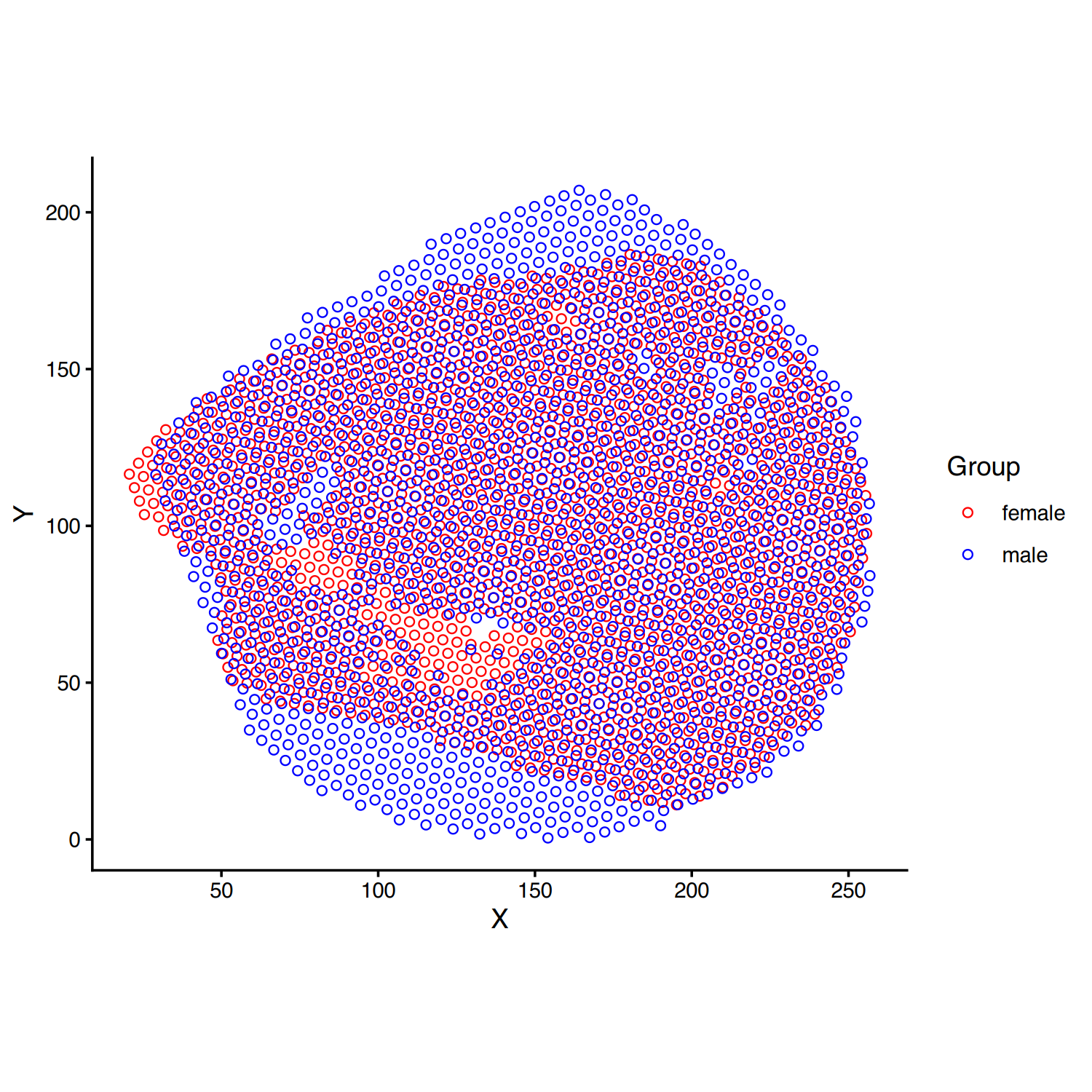
Although the two spatial transcriptomics datasets have been (very approximately) aligned, we still need to have a common spatial unit for comparison. As shown in the STcompare tutorial, to create a common spatial unit, we use rasterization via SEraster. This creates a one-to-one correspondence between measurements in one dataset to another despite slightly different numbers of cells/spots.
Again, I like to use visualization of the rasterized data to check that the rasterization is at a fine enough resolution as to not obscure spatial structures that we want to compare but also coarse enough to have more than one cell/spot per rasterization pixel to avoid 0s.
############# Create SpatialExperiment
female_genes <- setdiff(colnames(female_data), c("X", "Y"))
male_genes <- setdiff(colnames(male_data), c("X", "Y"))
shared_genes <- intersect(female_genes, male_genes)
length(shared_genes)

female_gexp <- female_data[, shared_genes]
female_spe <- SpatialExperiment::SpatialExperiment(
  assays = list(counts = t(female_gexp)),
  spatialCoords = as.matrix(female_pos[,1:2])
)
male_gexp <- male_data[, shared_genes]
male_spe <- SpatialExperiment::SpatialExperiment(
  assays = list(counts = t(male_gexp)),
  spatialCoords = as.matrix(male_pos[,1:2])
)

############# Rasterize
# interactively visualize and pick reasonable resolution
# to capture scale of molecular comparison
# and balance with runtime
resolution <- 15

spe_list <- list(female = female_spe, male = male_spe)
rast <- SEraster::rasterizeGeneExpression(
  spe_list,
  resolution = resolution,
  fun = "sum",
  square = FALSE,
  assay_name = "counts"
)

assay(rast$female, "CPM") <- Matrix::t(Matrix::t(assay(rast$female))/Matrix::colSums(assay(rast$female)))*1e6
assay(rast$male, "CPM") <- Matrix::t(Matrix::t(assay(rast$male))/Matrix::colSums(assay(rast$male)))*1e6

# visualize a gene as an example
g <- 'Aqp1'
p1 <- SEraster::plotRaster(rast$female, assay_name = "CPM", feature=g, name=g)
p2 <- SEraster::plotRaster(rast$male, assay_name = "CPM", feature=g, name=g)
p1 + p2
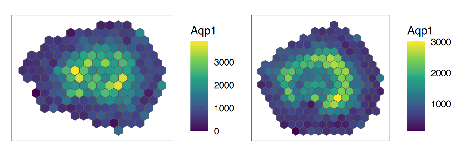
We are interested in spatial differential expression or changes in spatial pattern between our two samples. But one trivial way there could be a change is because a gene is spatially variable in one sample and not spatially variable in another. Using existing methods for identifying spatially variable genes can achieve this.
So, for demonstration purposes, we will actually filter out such genes so our STcompare analysis can focus on identifying genes that are spatially variable in both samples but change in their spatial patterning.
############# Identify SVGs
filter_dist <- 2 * resolution

w <- MERINGUE::getSpatialNeighbors(SpatialExperiment::spatialCoords(rast$female), filterDist = filter_dist)
MERINGUE::plotNetwork(SpatialExperiment::spatialCoords(rast$female), w)

moransI <- function(SE_temp, filterDist, assayName=1){

  # use MERINGUE to get the neighbor-relationships
  w <- MERINGUE::getSpatialNeighbors(SpatialExperiment::spatialCoords(SE_temp), filterDist = filterDist)
  par(mfrow=c(1,1))
  MERINGUE::plotNetwork(SpatialExperiment::spatialCoords(SE_temp), w)

  # Identify significantly spatially auto-correlated genes
  I <- MERINGUE::getSpatialPatterns(SummarizedExperiment::assays(SE_temp)[[assayName]], w)

  return(I)
}

moransI_female <- moransI(rast$female, filterDist = filter_dist, assayName = "CPM")
moransI_male <- moransI(rast$male, filterDist = filter_dist, assayName = "CPM")

svg_female <- moransI_female %>% filter(p.adj < 0.05) %>% rownames()
svg_male <- moransI_male %>% filter(p.adj < 0.05) %>% rownames()
svg_int <- intersect(svg_female, svg_male)

length(svg_int)
2069
This gives us 2069 genes that are spatially variable in both samples.
Similarly, to distinguish our STcompare analysis from what we could have discovered using more conventional differential expression analysis between the two samples, we will focus specifically on non-differentially expressed genes (p-value > 0.05 by a wilcox test) among our shared spatially variable genes.
############# Differential expression
genes_chosen <- svg_int

# just use simply wilcox test
dv <- sapply(genes_chosen, function(g) {
  wilcox.test(rast$female@assays@data$CPM[g,],
              rast$male@assays@data$CPM[g,])$p.value
})
names(dv) <- genes_chosen
dv <- p.adjust(dv, method = "BH")
hist(-log10(dv))

# focus on non-differentially expression geens
table(dv > 0.05)
FALSE  TRUE
 1760   309
This leaves us with only 309 genes that are spatially variable AND not differentially expressed at a bulk level between our samples.
nondg <- names(which(dv > 0.05))

input <- list('female' = rast$female[nondg, ],
              'male' = rast$male[nondg, ])
Now we’re ready to run STcompare’s spatial correlation analysis to identify genes that are spatially differentially expressed, which we define as significantly negatively spatially correlated.
The advance presented in STcompare is that such a statistical evaluation needs to control for the spatial autocorrelation common to spatial transcriptomics data in order to mitigate false positives. To control for such autocorrelation, we need to choose a series of bandwidths that are evaluated.
The tutorial used a range of bandwidths that were too small given the number of raster pixels due to my choice of a rather coarse rasterization resolution. At this stage, I could’ve either gone back and chosen a finer rasterization resolution or remove certain small bandwidths from the evaluation. I went with the latter.
Note this bug persists in the vibed code, which perhaps speaks to how we should update the package to catch such errors and/or provide more documentation to inform students and AI agents alike in the first place.
############# Spatial Correlation
# Omit delta 0.01: with ~100 raster pixels, nn=0.01 is ~1 neighbor and
# locfit overflows the C stack. Be mindful of smallest safe bandwidth.
deltaList <- replicate(length(nondg), seq(0.1, 0.9, .1), simplify = FALSE)
nPermutations <- c(100, 1000)

kidneyCorrelation <- STcompare::spatialCorrelationGeneExpIterPermutations(
  input,
  nPermutations = nPermutations,
  deltaX = deltaList,
  deltaY = deltaList,
  assayName = "CPM",
  nThreads = 10,
  verbose = TRUE,
  seed = 0
)
head(kidneyCorrelation)
       correlationCoef  pValueNaive pValuePermuteX pValuePermuteY
Adhfe1      0.31096974 2.961203e-05    0.000000000     0.02942857
Ptpn18      0.21221641 4.935049e-03    0.087288136     0.04598214
Hs6st1      0.45289083 3.505580e-10    0.003814815     0.00000000
Mgat4a      0.38230095 1.933061e-07    0.003814815     0.00000000
Myo1b       0.37970407 2.373897e-07    0.000000000     0.00000000
Clk1        0.06880476 3.669904e-01    0.478075472     0.50108108
       deltaStarMedianX deltaStarMedianY   deltaStarX
Adhfe1             0.20              0.2 0.3, 0.5....
Ptpn18             0.50              0.3 0.4, 0.5....
Hs6st1             0.60              0.5 0.9, 0.9....
Mgat4a             0.40              0.4 0.6, 0.5....
Myo1b              0.60              0.5 0.3, 0.9....
Clk1               0.45              0.5 0.4, 0.9....
         deltaStarY nullCorrelationsX nullCorrelationsY
Adhfe1 0.2, 0.2....      -0.07395....      0.089810....
Ptpn18 0.3, 0.1....      -0.18817....      -0.00688....
Hs6st1 0.4, 0.9....      -0.19994....      -0.22322....
Mgat4a 0.3, 0.5....      -0.21264....      -0.08971....
Myo1b  0.9, 0.9....      -0.13572....      -0.12305....
Clk1   0.4, 0.5....      -0.18703....      -0.03509....
Now we can filter for the genes that have significant negative spatial correlation while controlling for autocorrelation.
svgSigNeg <- kidneyCorrelation %>%
  dplyr::filter(pValuePermuteX < 0.2 | pValuePermuteY < 0.2) %>%
  dplyr::filter(correlationCoef < 0) %>%
  rownames()
kidneyCorrelation[svgSigNeg,]
        correlationCoef  pValueNaive pValuePermuteX
Des          -0.1169080 0.1244697822      0.2586344
Slco1a6      -0.2766732 0.0002193068      0.1650000
        pValuePermuteY deltaStarMedianX deltaStarMedianY
Des         0.14644550              0.4              0.5
Slco1a6     0.06717391              0.1              0.6
          deltaStarX   deltaStarY nullCorrelationsX
Des     0.1, 0.1.... 0.4, 0.5....      -0.04003....
Slco1a6 0.3, 0.9.... 0.4, 0.9....      -0.30683....
        nullCorrelationsY
Des          0.026257....
Slco1a6      -0.13325....
There are very few genes (only 2!) meeting this criteria. If we look at one of the genes corresponding to a solute carrier, we can appreciate that this gene is indeed spatially variable in both, not significantly differentially expressed in bulk, but exhibits a different spatial pattern in the male vs female kidney.
g <- "Slco1a6"
dv[g] # differential expression p-value
0.100163
moransI_female[g,] # signicantly spatially variable
         observed     expected        sd p.value p.adj
Slco1a6 0.5841242 -0.005747126 0.0450336       0     0
moransI_male[g,] # signicantly spatially variable
         observed     expected         sd p.value p.adj
Slco1a6 0.5144665 -0.004975124 0.04169797       0     0
p1 <- SEraster::plotRaster(rast$female, assay_name = "CPM", feature_name = g, name = g)
p2 <- SEraster::plotRaster(rast$male, assay_name = "CPM", feature_name = g, name = g)
p1 + p2
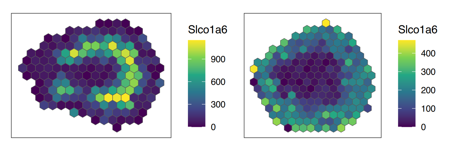
I was curious if this differential spatial patterning was shared by other solute carriers. So to just visually check some other solute carriers, I grepped for other Slc prefix genes as a quick look.
intersect(
  colnames(female_data)[grepl('Slc', colnames(female_data))],
  svgSigPos
)
 [1] "Slc23a3"  "Slco4a1"  "Slc2a2"   "Slc16a4"  "Slc39a8"
 [6] "Slc35a1"  "Slc2a1"   "Slc2a5"   "Slc1a5"   "Slc22a18"
[11] "Slc10a2"  "Slc25a15" "Slc19a1"  "Slc1a4"   "Slc22a5"
[16] "Slc9a3r1" "Slc6a19"  "Slc7a7"   "Slc15a2"  "Slc5a3"
[21] "Slc14a2"  "Slc22a8"  "Slc35g1"  "Slc16a2"
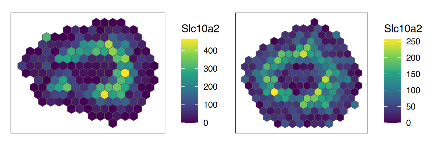
A cherry picked a few to compare the STcompare statistics and visually assess.
g <- "Slc10a2"
p1 <- SEraster::plotRaster(rast$female, assay_name = "CPM", feature_name = g, name = g)
p2 <- SEraster::plotRaster(rast$male, assay_name = "CPM", feature_name = g, name = g)
p1 + p2
kidneyCorrelation[g,]
        correlationCoef  pValueNaive pValuePermuteX
Slc10a2       0.5539799 2.204791e-15              0
        pValuePermuteY deltaStarMedianX deltaStarMedianY
Slc10a2              0              0.1              0.1
          deltaStarX   deltaStarY nullCorrelationsX
Slc10a2 0.5, 0.2.... 0.1, 0.9....      0.137984....
        nullCorrelationsY
Slc10a2      0.249081....
g <- "Slc5a3"
p1 <- SEraster::plotRaster(rast$female, assay_name = "CPM", feature_name = g, name = g)
p2 <- SEraster::plotRaster(rast$male, assay_name = "CPM", feature_name = g, name = g)
p1 + p2
kidneyCorrelation[g,]
       correlationCoef  pValueNaive pValuePermuteX pValuePermuteY
Slc5a3       0.7695974 2.436148e-35              0              0
       deltaStarMedianX deltaStarMedianY   deltaStarX
Slc5a3              0.3              0.3 0.7, 0.2....
         deltaStarY nullCorrelationsX nullCorrelationsY
Slc5a3 0.2, 0.2....      -0.50409....      -0.52759....
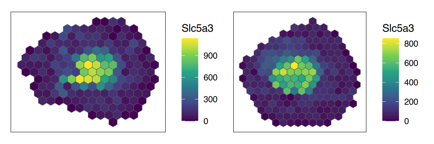
Indeed, these genes are significantly positively spatially correlated (not negatively). So the significant negative spatial correlation for Slco1a6 is not necessarily shared by other solute carriers.
In the mouse kidney, Slco1a6 (Solute carrier organic anion transporter family member 1A6, also known as OATP1A6 or Oatp5) is known to exhibit strong sexual dimorphism. The human ortholog is SLCO1A2. I wonder if this gene is also sexually dimorphic in human kidneys and ultimately what the differences in the spatial organization of this solute carrier means in terms of functional consequences in kidney health for men and women?
Try it out for yourself
- Download the data and run through this pipeline yourself.
- What happens if you perform a diffeomorphic or spline-based alignment instead of just a simple affine?
- What happens if you rasterize at a finer resolution? A coarser resolution?
- Given this now well-defined code pipeline, can you constrain an AI agent to evaluate a number of new datasets with the appropriate parameter sweeps? How can you define what is ‘appropriate’ without iterative interactive visualization and intervention from you?
Recent Posts
- STcompare to identify spatially sexually dimorphic genes in mouse kidneys on 22 September 2026
- AI-guided data visualization of gas prices in different geographical locations across the US over time on 04 May 2026
- The Mentorship Index on 01 March 2026
- Vibe coding with SEraster and STcompare to compare spatial transcriptomics technologies on 22 February 2026
- RNA velocity in situ infers gene expression dynamics using spatial transcriptomics data on 13 October 2025