Introduction

We recently developed a reference-free deconvolution approach for analyzing multi-cellular pixel-resolution spatially resolved transcriptomics data called STdeconvolve now published in Nature Communications. STdeconvolve recovers the proportion of cell types comprising each multi-cellular spatially resolved pixel along with each cell types’ putative transcriptional profile without reliance on external single-cell transcriptomics references. More details regarding how the method works and demonstrations of its application to diverse spatially resolved transcriptomics datasets and technologies can be found in the published paper as well as on https://jef.works/STdeconvolve/. STdeconvolve is implemented as an R software package available on Github at https://github.com/JEFworks-Lab/STdeconvolve and on Bioconductor.

In this blog post, I will explore the difference between deconvolution analysis as enabled by STdeconvolve compared to clustering analysis on the multi-cellular pixels. I hope this story will be a fun demonstration of the differences between these two different analysis approaches for the same multi-cellular resolution spatially resolved transcriptomics data.

The data

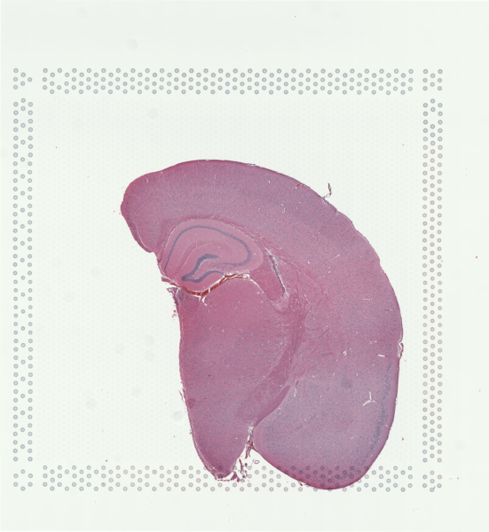
For demonstration purposes in this blog post, let’s use a publicly available Visium dataset of an FFPE preserved adult mouse brain partial coronal section from 10X Genomics.

## read in pixel position information
pos.info <- read.csv('adult-mouse-brain-ffpe-1-standard-1-3-0/spatial/tissue_positions_list.csv', header=FALSE)
pos <- pos.info[,c(6,5)]
rownames(pos) <- pos.info[,1]
colnames(pos) <- c('x', 'y')
plot(pos)

## read in gene expression counts
cd <- Matrix::readMM('adult-mouse-brain-ffpe-1-standard-1-3-0/filtered_feature_bc_matrix/matrix.mtx.gz')
barcodes <- read.csv('adult-mouse-brain-ffpe-1-standard-1-3-0/filtered_feature_bc_matrix/barcodes.tsv.gz', sep='\t', header=FALSE)
features <- read.csv('adult-mouse-brain-ffpe-1-standard-1-3-0/filtered_feature_bc_matrix/features.tsv.gz', sep='\t', header=FALSE)
rownames(cd) <- features[,2]
colnames(cd) <- barcodes[,1]
cd[1:5,1:5]

## restrict to only pixels with genes
## and flip right side up
pos <- pos[colnames(cd),]
pos[,2] <- -pos[,2]

As we’ve previously reviewed in our Nature Communications commentary, Visium is one of the spatial transcriptomic (ST) technologies that have enabled non-targeted, genome-wide transcriptional profiling at pixel resolution.

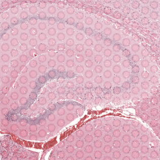
Zooming into this corresponding histology image, we can confirm visually that some ST pixels do indeed cover multiple cells. As such, the measured gene expression at these ST pixels will be an aggregate of the gene expression from all the covered cells, which may represent multiple cell types.

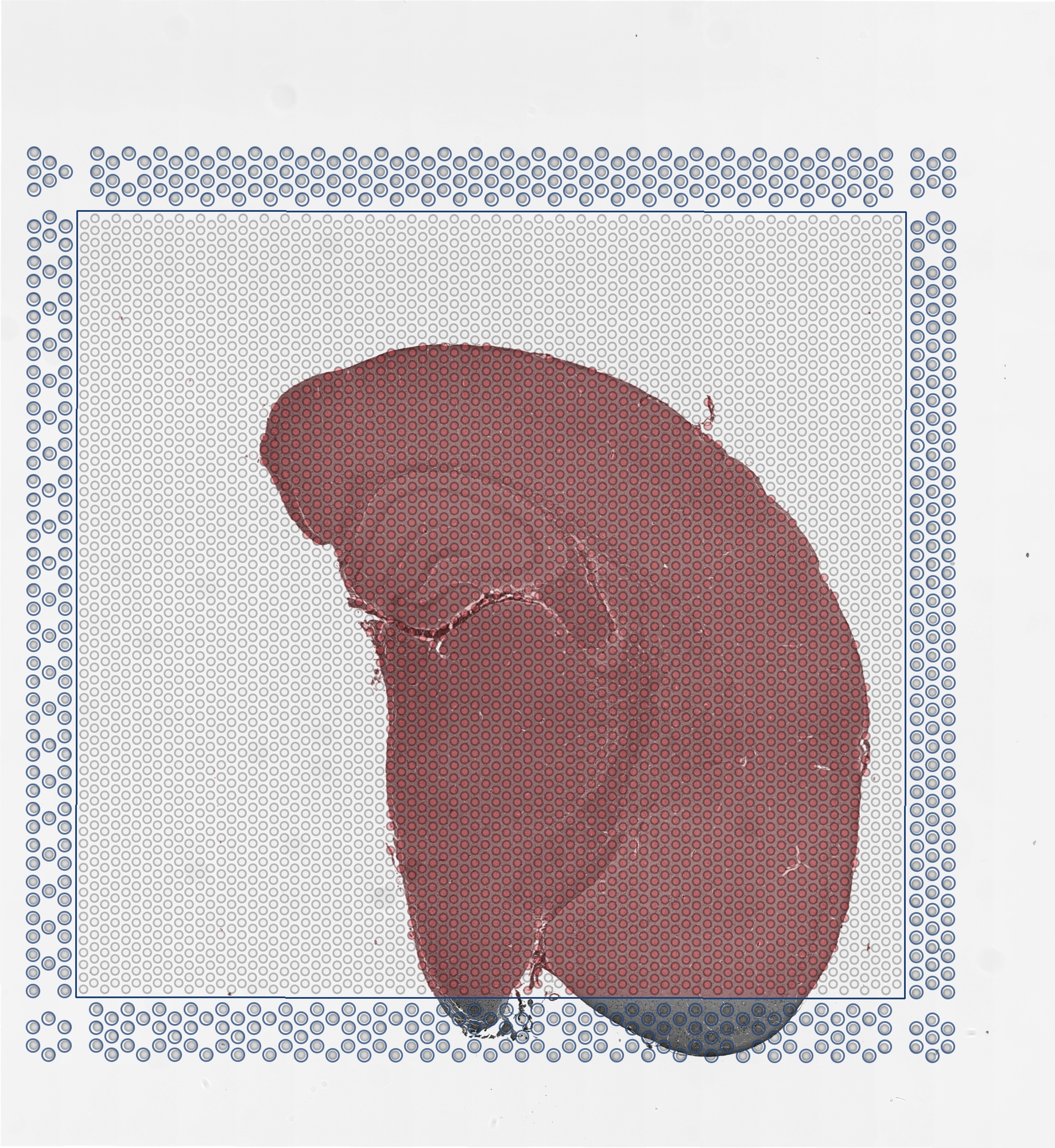
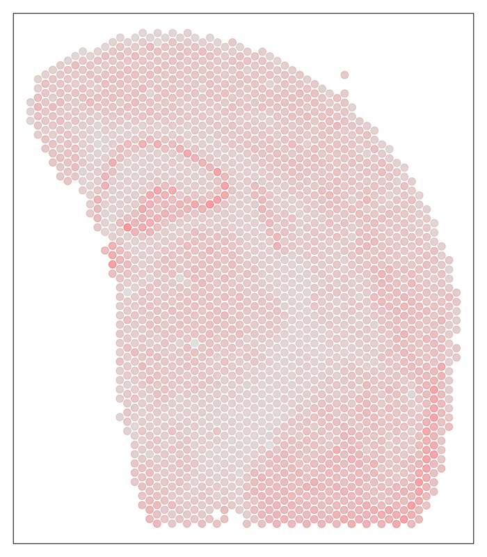
We can further visualized these ST pixels and the total number of genes detected per pixel to get a sense of the structure in the data that we’ll be tinkering with.

## visualize depth
par(mfrow=c(1,1), mar=rep(1,4))
MERINGUE::plotEmbedding(pos, col=colSums(cd), cex=1)

Deconvolution analysis with STdeconvolve

Since each ST pixel comprises multiple cells that may correspond to multiple cell types, we will apply STdeconvolve to recover the proportion of cell types comprising each multi-cellular spatially resolved pixel along with each cell type’s putative transcriptional profile.

library(STdeconvolve)
## remove pixels with too few genes
counts <- STdeconvolve::cleanCounts(cd, 
                                    min.lib.size = 1, 
                                    max.lib.size = Inf,
                                    min.reads = 2000, 
                                    verbose = TRUE)

## feature select for genes
corpus <- STdeconvolve::restrictCorpus(counts, 
                                       removeAbove=1.0, 
                                       removeBelow = 0.05,
                                       alpha = 0.01,
                                       nTopOD = NA)
dim(corpus)

## choose number of cell types
ldas <- STdeconvolve::fitLDA(t(as.matrix(corpus)), Ks = c(12))

## get best model results
optLDA <- STdeconvolve::optimalModel(models = ldas, opt = 12)

## extract deconvolved cell type proportions (theta) and transcriptional profiles (beta)
results <- STdeconvolve::getBetaTheta(optLDA, 
                                      perc.filt = 0.05, 
                                      betaScale = 1000)
deconProp <- results$theta
deconGexp <- results$beta

## normalize for comparison purposes later
matdecon <- MERINGUE::normalizeCounts(t(deconGexp), log=FALSE, depthScale = 1000)

Clustering analysis

Alternatively, we can just perform clustering analysis on the ST pixels. For comparative purposes, we will restrict to the same set of genes used in deconvolution and normalize in a similar manner. Then we will apply principal components dimensionality reduction and do graph-based community detection as if these pixels were single cells much like in a clustering analysis for single cell RNA-seq data.

## restrict to same genes and normalize in same way
matsub <- MERINGUE::normalizeCounts(cd[rownames(matdecon),], log=FALSE, depthScale = 1000)

## PCA
pcs <- prcomp(t(matsub))
pcs1 <- pcs$x

## look at variance explained to pick reasonable number of PCs
#plot(pcs$sdev[1:50], type="l")

## graph-based community detection with Louvain
set.seed(0)
com <- MUDAN::getComMembership(pcs1[,1:30], k=30, 
                               method=igraph::cluster_louvain)

For comparative purposes, we will also project the normalized deconvolved gene expression profiles for cell types from STdeconvolve into the same PC space by applying the same set of PC loadings for visualization later.

## project to same PCs
pcs2 <- t(matdecon) %*% pcs$rotation
#dim(pcs1)
#dim(pcs2)

## combine into one PC matrix
pcsall <- as.matrix(rbind(pcs1[,1:30], pcs2[,1:30]))

This way, we will be able to generate a 2D UMAP embedding using the top PCs from both the observed gene expression profile for each ST pixel as well as the deconvolved gene expression profile for each cell type from STdeconvolve.

## UMAP
set.seed(0)
emb <- uwot::umap(pcsall, 
                  n_neighbors=30, min_dist=0.1)
rownames(emb) <- c(rownames(pcs1), rownames(pcs2))

Let’s visualize and compare

Now we’re ready to visualize and compare the results from our two different analyses. To enhance the saliency of our comparison, let’s try to match up the colors of the ST pixel clusters identified through clustering analysis and the cell types identified through deconvolution analysis by STdeconvolve.

We will create a pseudobulk gene expression profile for the ST pixel clusters identified through clustering analysis.

## make model matrix
mm <- model.matrix(~ 0 + com)
colnames(mm) <- levels(com)
matmatch <- cd %*% mm
matmatch <- MERINGUE::normalizeCounts(matmatch[matsub,], log=FALSE, depthScale = 1000)

And then correlate the pseudobulk gene expression profile for the ST pixel clusters with our deconvolved gene expression profiles for cell types from STdeconvolve.

## correlate gene expression
cmat <- cor(as.matrix(matmatch), as.matrix(matdecon))

We will use a Hungarian sort algorithm to help match up each ST pixel cluster with each deconvolved cell type based on transcriptional similarity (e.g. high correlation).

## optimal transcriptional match 
## based on Hungarian sort
hsort <- STdeconvolve::lsatPairs(cmat)
match <- hsort$colsix
names(match) <- hsort$rowix

And now we can color each ST pixel cluster and their corresponding best transcriptionally matched deconvolved cell type (and vice versa) with the same colors.

## set common colors
cols <- MERINGUE:::fac2col(names(match),
                           level.colors = RColorBrewer::brewer.pal(12, 'Paired'))
names(cols) <- names(match)
cols
cols2 <- cols
names(cols2) <- match
cols2 <- cols2[colnames(matdecon)]
names(cols2) <- colnames(matdecon)
## manually change some colors due to close matches
cols2[1] <- cols[4]
cols2[4] <- cols[3]
cols2[2] <- 'lightgrey'

We can use a heatmap to visualize these transcriptional correspondences between ST pixel clusters and deconvolved cell types and their assigned colors.

## heatmap of correlation matrix
heatmap(cmat[names(match), union(match, colnames(matdecon))], 
        scale='none', Rowv=NA, Colv=NA,
        RowSideColors = cols,
        ColSideColors = cols2[union(match, colnames(matdecon))],
        col=colorRampPalette(c('blue', 'white', 'red'))(100),
        xlab = 'Deconvolved Cell Types',
        ylab = 'Pixel Clusters')

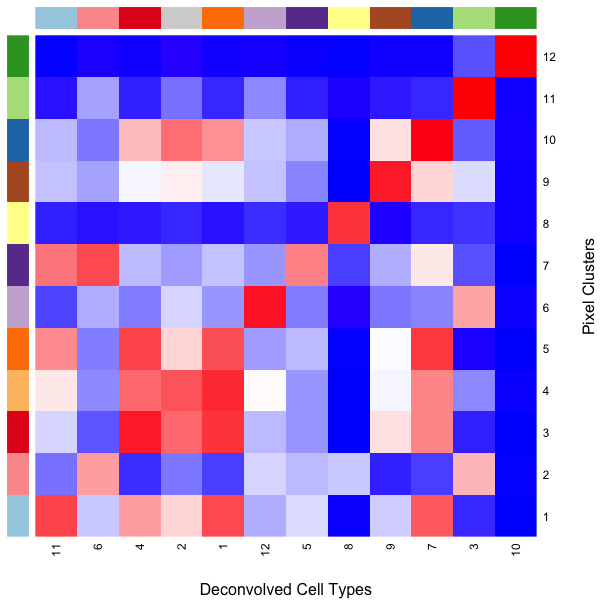
So we can see here that deconvolved cell type 10 transcriptionally strongly correlates with pixel cluster 12 and are both assigned to the color dark green for example.

Deconvolution analysis results

Now, let’s visualize the deconvolution analysis results from STdeconvolve! We can visualized the deconvolved cell types on the UMAP embedding as well as on the original tissue using little pie charts to represent their proportional composition in each pixel.

In the UMAP embedding, to distinguish the pixels from the deconvolved cell types (since both are included in the same embedding), we will increase the alpha of the points corresponding to ST pixels to make them more transparent and circle/label the deconvolved cell types to highlight them more clearly.

## plot deconvolved cell types
MERINGUE::plotEmbedding(emb, groups=com, group.level.colors = cols, cex=0.5, mark.clusters=FALSE, alpha=0.05) 
points(emb[colnames(matdecon),], cex=3, col=cols2, lwd=2)
text(emb[colnames(matdecon),], labels=colnames(matdecon))

plt <- vizAllTopics(deconProp, pos, lwd = 0,
             r=100, topicCols = cols2, topicOrder = names(cols2))  +
  ggplot2::guides(fill=ggplot2::guide_legend(ncol=2)) +
  ggplot2::guides(colour = "none")
plt 

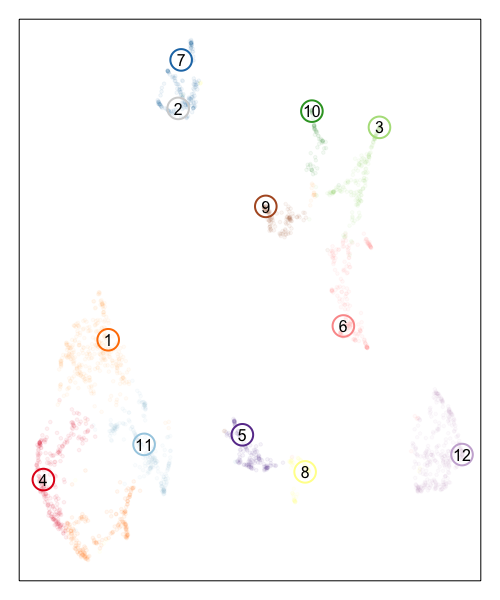
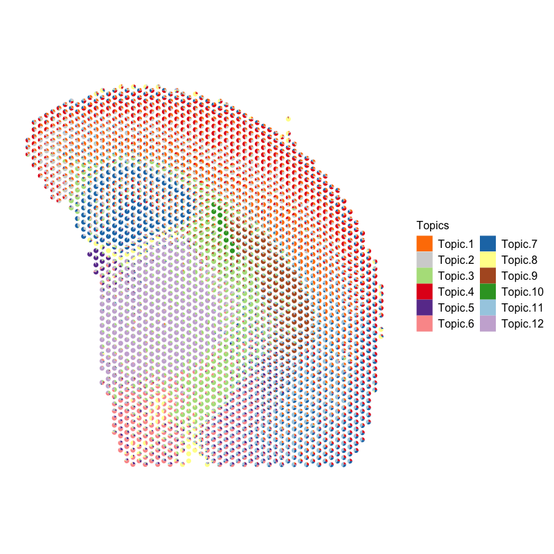
Based on the visualization of the deconvolved cell types on the tissue spatial coordinates, we can see how different cell types are spatially organized in distinct domains and structures as expected!

Clustering analysis results

Now, let’s visualize the clustering analysis results! We can visualize both the ST pixel clusters on the UMAP embedding as well as on the original tissue. We will label the ST pixel cluster numbers in both the UMAP embedding and on the tissue.

## plot pixels
par(mfrow=c(1,2), mar=rep(1,4))
MERINGUE::plotEmbedding(emb, groups=com, group.level.colors = cols, cex=0.5, mark.clusters=TRUE, mark.cluster.cex = 1) 
MERINGUE::plotEmbedding(pos, groups=com, group.level.colors = cols, cex=1, mark.clusters=TRUE) ## on tissue

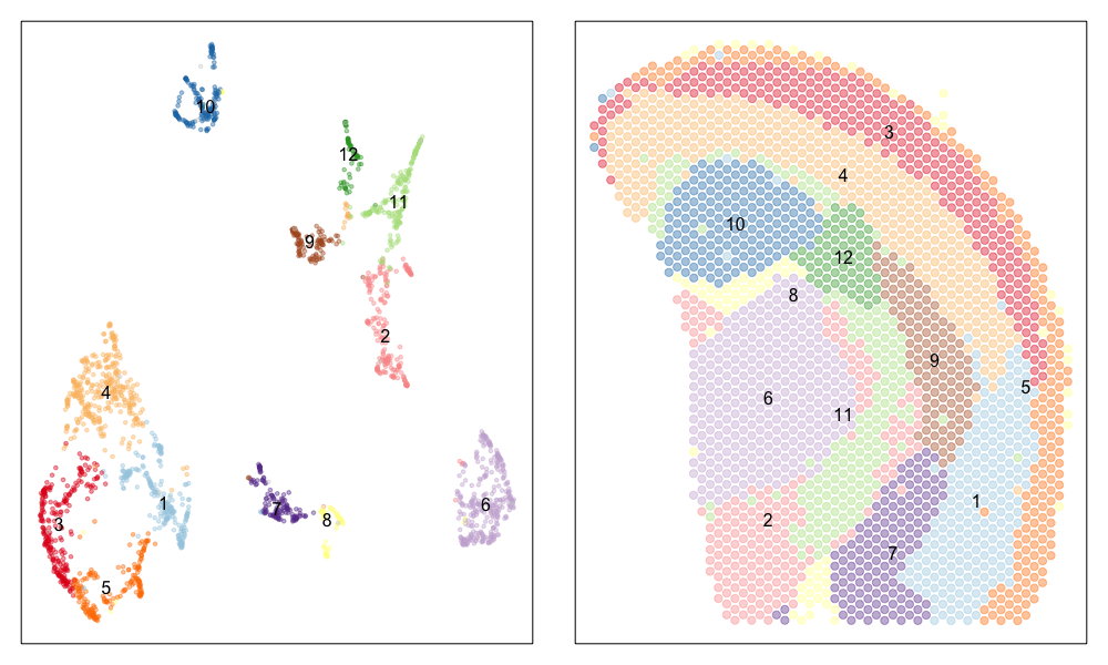
We can indeed identify many transcriptionally distinct clusters of ST pixels. When we visualize these clusters on the tissue spatial coordinates, we can still see how different transcriptionally distinct clusters of ST pixels are spatially organized in distinct domains and structures.

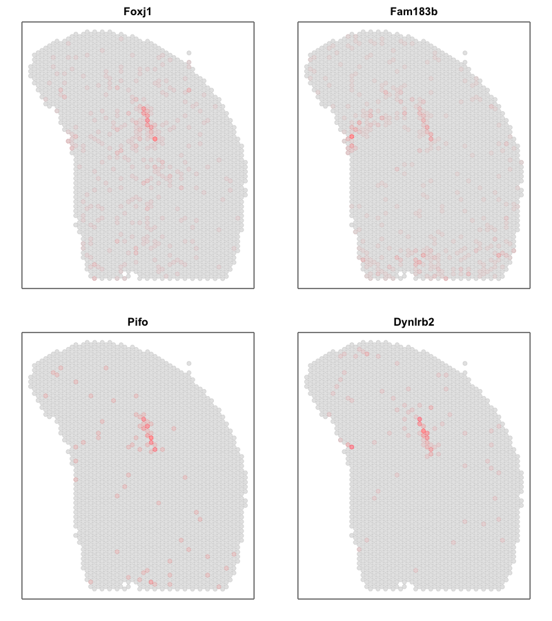
Interestingly, the spatial positions of the ST pixel clusters do visually match reasonably well with the proportional representation of the transcriptionally corresponding deconvolved cell types! For example, we saw previously that deconvolved cell type 10 transcriptionally strongly correlates with pixel cluster 12 (both dark green) and both are spatially localized to the same region. We can perhaps further reference a map like The Allen Brain Atlas coronal map and integrate other knowledge to suggest that perhaps deconvolved cell type 10 (in dark green) corresponds to ependymal cells lining the lateral ventricle for example. We can further visualize putative ependymal cell marker genes and see that these marker genes indeed are highly expressed in the same tissue regions.

## ependymal marker genes
gs <- c('Foxj1', 'Fam183b', 'Pifo', 'Dynlrb2')
par(mfrow=c(2,2), mar=rep(2,4))
sapply(gs, function(g) {
  MERINGUE::plotEmbedding(pos, col=cd[g,], cex=.5, main=g)
})

What do you think? What are some similarities and differences between the two analysis for this same dataset?

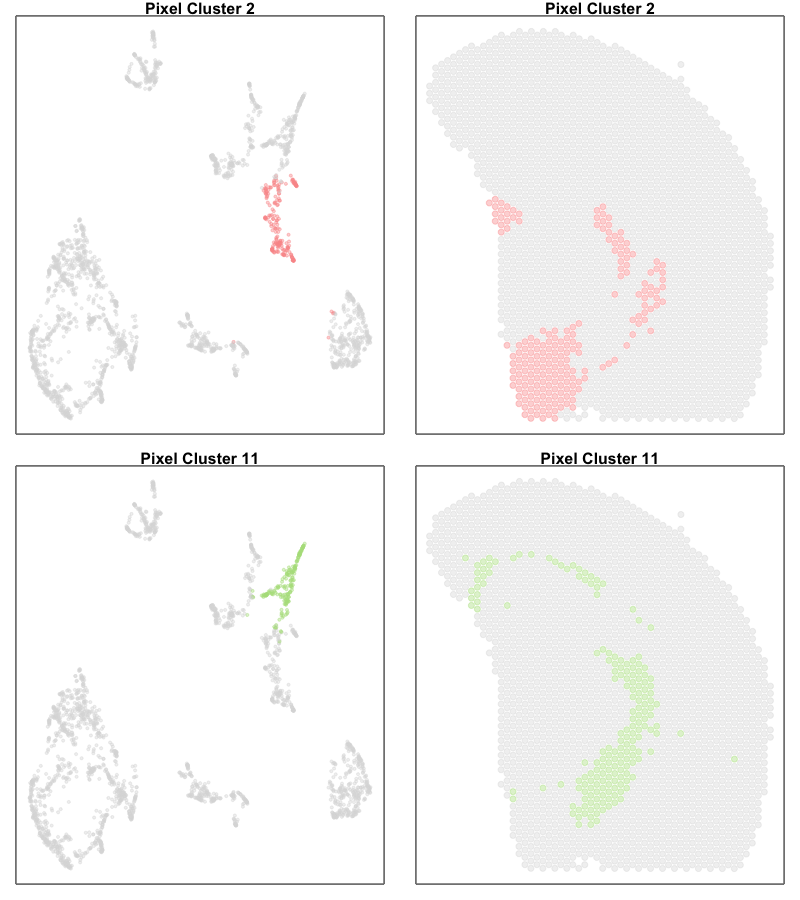
Trajectory or cell type mixture?

One potential difference made more salient in our joint UMAP embedding is that the ST pixels can sometimes form what looks like trajectories. For example, there appears to be a trajectory going from ST pixel cluster 2 to 11.

In true single-cell resolution analysis, such a trajectory may suggest the existance of transcriptionally intermediate cell-states along a dynamic process.

par(mfrow=c(2,2))
vi <- com %in% c(2)
MERINGUE::plotEmbedding(emb[rownames(deconProp),], groups=com[vi], group.level.colors = cols, main='Pixel Cluster 2', cex=0.5,
                        unclassified.cell.color = '#dddddd')
MERINGUE::plotEmbedding(pos, groups=com[vi], group.level.colors = cols, main='Pixel Cluster 2', cex=1,
                        unclassified.cell.color = '#dddddd')
vi <- com %in% c(11)
MERINGUE::plotEmbedding(emb[rownames(deconProp),], groups=com[vi], group.level.colors = cols, main='Pixel Cluster 11', cex=0.5,
                        unclassified.cell.color = '#dddddd')
MERINGUE::plotEmbedding(pos, groups=com[vi], group.level.colors = cols, main='Pixel Cluster 11', cex=1,
                        unclassified.cell.color = '#dddddd')

However, projecting our deconvolved cell types into the same UMAP embedding, we only identify deconvolved cell types 6 and 3 as corresponding to the terminal states along this ‘trajectory’. If we further visualize the deconvolved cell type proportions for deconvolved cell types 6 and 3, we see that this ‘trajectory’ may actually be made up of differing mixtures of these two cell types. That is, rather than individual single cells changing their transcriptional states along a dynamic process, this ‘trajectory’ may be driven by differing proportions of two different cell-types in these multi-cellular ST pixels.

par(mfrow=c(2,2))
MERINGUE::plotEmbedding(emb[rownames(deconProp),], col=deconProp[, 6], main='Deconvolved cell type 6', cex=0.5,
                        gradientPalette = colorRampPalette(c('#dddddd', cols2[6]))(100))
points(t(as.matrix(emb['6',])), cex=3, col=cols2[6], lwd=2)
text(t(as.matrix(emb['6',])), labels='6')
MERINGUE::plotEmbedding(pos, col=deconProp[, 6], main='Deconvolved cell type 6', cex=1,
                        gradientPalette = colorRampPalette(c('#dddddd', cols2[6]))(100))

MERINGUE::plotEmbedding(emb[rownames(deconProp),], col=deconProp[, 3], main='Deconvolved cell type 3', cex=0.5,
                        gradientPalette = colorRampPalette(c('#dddddd', cols2[3]))(100))
points(t(as.matrix(emb['3',])), cex=3, col=cols2[3], lwd=2)
text(t(as.matrix(emb['3',])), labels='3')
MERINGUE::plotEmbedding(pos, col=deconProp[, 3], main='Deconvolved cell type 3', cex=1,
                        gradientPalette = colorRampPalette(c('#dddddd', cols2[3]))(100))

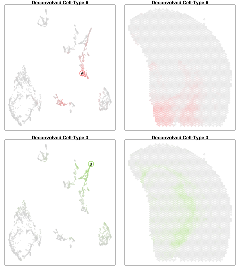
Perhaps another good reminder to always follow up on the hunches a visualization gives you (in this case that there is a cellular trajectory) and interpret these visualizations in the context of the underlying data (in this case, multicelluar pixels that may comprise multiple cell types)!

Try it out for yourself!

• There are single-cell resolution targeted spatially resolved transcriptomics data of similar tissue (coronal section of the adult mouse brain) available. Could we use these to help validate our suspicion that these are not true cellular trajectories but different mixtures of cell types?
• There are many public multi-cellular pixel-resolution spatially resolved transcriptomics datasets available. See if you can compare clustering versus deconvolution on your own.