Annotating STdeconvolve Cell-Types with ASCT+B Tables
Introduction
We recently published a reference-free deconvolution approach for
analyzing multi-cellular pixel-resolution spatially resolved
transcriptomics data called
STdeconvolve.
When applied to multi-cellular pixel-resolution spatially resolved
transcriptomics data, STdeconvolve can recover the proportion of cell
types comprising each spatially resolved pixel along with each cell
types’ putative transcriptional profile without reliance on external
single-cell RNA-seq references.
A common question I’ve encountered from students is: “without an annotated reference single-cell RNA-seq dataset, how do I annotate the deconvolved cell types?” While I generally recommend consulting a biological domain expert (or referencing primary literature towards become a biological domain expert yourself!) for annotating cell-types, in this blog post, I will demonstrate how we can take a data-driven approach using biological domain expert curated genesets from HuBMAP’s ASCT+B Tables as a first pass.
Pixel-resolution spatial transcriptomics data of the lymph node
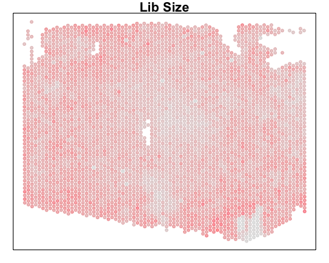
For demonstration purposes in this blog post, let’s use a publicly available Visium dataset of a lymph node from 10X Genomics. We can read in the pixel-resolution gene expression measurements along with the spatial positions of the pixels. As a preliminary look at the data, we can visualize the total number of genes detected per pixel.
library(Matrix)
## gene expression
gexp <- Matrix::readMM('human-lymph-node-1-standard-1-1-0/filtered_feature_bc_matrix/matrix.mtx.gz')
barcodes <- read.csv('human-lymph-node-1-standard-1-1-0/filtered_feature_bc_matrix/barcodes.tsv.gz', header=FALSE)
features <- read.table('human-lymph-node-1-standard-1-1-0/filtered_feature_bc_matrix/features.tsv.gz', header=FALSE)
colnames(gexp) <- barcodes[,1]
rownames(gexp) <- features[,2]

## spatial positions of pixels
posinfo <- read.csv('human-lymph-node-1-standard-1-1-0/spatial/tissue_positions_list.csv', header=FALSE)
pos <- posinfo[,5:6]
rownames(pos) <- posinfo[,1]
### restrict to same set
pos <- pos[colnames(gexp),]

## plot pixels and total genes detected
par(mfrow=c(1,1), mar=rep(1,4))
MERINGUE::plotEmbedding(pos, col=Matrix::colSums(gexp), main='Lib Size')
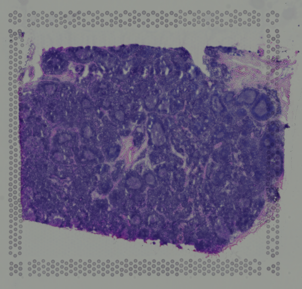
We can also take a look at the corresponding H&E staining image. In this case, even visually, we can see some interesting histological patterns that a skilled pathologist would be able to use to identify certain cell types. For example, we can see these circular structures that correspond to the germinal centers. We will reference these histological patterns and known cell type spatial localization patterns to double check our data-driven cell type annotations later.
As we’ve seen in previous tutorials, some pixels cover multiple cells. As such, the measured gene expression at these pixels will be an aggregate of the gene expression from all the covered cells, which may represent multiple cell types. Deconvolution analysis can allow us to deconvolve the relative gene expression contributions of each cell types in these multi-cellular pixels.
Analysis with STdeconvolve
So let’s analyze the dataset with deconvolution analysis using
STdeconvolve. We will generally follow the main
STdeconvolve vignette.
library(STdeconvolve)
## remove pixels with too few genes
counts <- cleanCounts(gexp, min.lib.size = 4000)
## filter pos to same set of pixels
pos2 <- pos[colnames(counts),]
colnames(pos2) <- c('x', 'y')
## feature select for genes
corpus <- restrictCorpus(counts, removeAbove=1.0, removeBelow = 0.05, nTopOD = NA)
## choose optimal number of cell-types
### previously ran with sequence to identify K=14 as optimum
#ldas <- fitLDA(t(as.matrix(corpus)), Ks = seq(5, 15, by = 1))
### just run K=14 for vignette building
ldas <- fitLDA(t(as.matrix(corpus)), Ks = c(14))
## get best model results
optLDA <- optimalModel(models = ldas, opt = "min")
## extract deconvolved cell-type proportions (theta) and transcriptional profiles (beta)
results <- getBetaTheta(optLDA, perc.filt = 0.05, betaScale = 1000)
deconProp <- results$theta
deconGexp <- results$beta
## color deconvolved topics based on transcriptional similarity
hc <- hclust(dist(deconGexp), 'ward.D2')
topicCols <- rainbow(nrow(deconGexp))
names(topicCols ) <- rownames(deconGexp)[hc$order]
topicCols <- topicCols [rownames(deconGexp)]
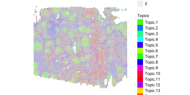
## visualize deconvolved cell-type proportions
vizAllTopics(deconProp, pos2,
topicCols=topicCols,
r=50, lwd = 0.05)
Given the large number of deconvolved cell types, we can visualized the proportion of each deconvolved cell type in pixels as separate plots.
gs <- lapply(1:ncol(deconProp), function(i) {
  g1 <- vizTopic(theta = deconProp, pos = pos2,
         topic = i, plotTitle = paste0('topic ', i),
         size = 1, stroke = 0.05, alpha = 1,
         low = "white",
         high = topicCols[i],
         showLegend = FALSE)
  return(g1)
})
library(gridExtra)
do.call("grid.arrange", c(gs, ncol=4))
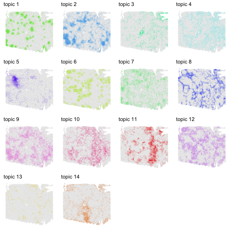
Visually, we can already see some interesting spatial patterns for these deconvolved cell types! For example, deconvolved cell type 1 appear to form these circular structures. Let’s look more into what these deconvolved cell types may be.
Annotating deconvolved cell types with ASCT+B Tables
To annotate our deconvolved cell types, we will integrate information from the Anatomical Structures, Cell Types, plus Biomarkers (ASCT+B) tables from the HuBMAP consortia. We will download the appropriate ASCT+B table for lymph node based on our tissue being analyzed. A quick look at the table contents shows each row as a cell type that is annotated by biological domain experts with references provided.
############ ASCT+B table
asctb <- read.csv('ASCT-B_NIH_Lymph_Node.csv', skip = 10)
asctb[1:2,]
##         AS.1 AS.1.LABEL        AS.1.ID    AS.2            AS.2.LABEL
## 1 lymph node lymph node UBERON:0000029 Capsule capsule of lymph node
## 2 lymph node lymph node UBERON:0000029 Capsule capsule of lymph node
##          AS.2.ID      AS.3              AS.3.LABEL        AS.3.ID AS.3.NOTES
## 1 UBERON:0002194
## 2 UBERON:0002194 Arteriole arteriole of lymph node UBERON:8410042
##   AS.4 AS.4.LABEL AS.4.ID AS.4.NOTES AS.5 AS.5.LABEL AS.5.ID
## 1
## 2
##                            CT.1                    CT.1.LABEL    CT.1.ID
## 1                 Myofibroblast            myofibroblast cell CL:0000186
## 2 Blood Vessel Endothelial Cell blood vessel endothelial cell CL:0000071
##   CT.1.NOTES
## 1
## 2
##                           All.Protein.Biomarkers.from.Antibody.Based.Assays.IHC..FACS
## 1 Collagen I+, Collagen III+, Elastin+, Desmin+/-, Smooth Muscle Actin+, Vimentin +/-
## 2                           CD31+, CD34+, CD59+, CD105+, CD144+, Podoplanin-, PROX-1-
##                                                                                                                                                                   Transcriptomics.With.References
## 1                                                                                                                                                                 ACTA2, COL1A1, COL3A1 Predicted
## 2 CAV1, CCL14, CD34, CD74, CD209, CD300LG, DARC, EMCN, ESAM, ICAM1, JAM2, HLA-DRA, HLA-DRB1, HLA-DPA1, HLA-DPB1, MARCO, PLVAP, PVRL2, SPARCL1, PECAM1 inferred general signature from Takeda 2020
##   BGene.1 BGene.1.LABEL BGene.1.ID BGene.2 BGene.2.LABEL BGene.2.ID BGene.3
## 1   ACTA2         ACTA2   HGNC:130  COL1A1        COL1A1 HGNC: 2197  COL3A1
## 2    CAV1          CAV1  HGNC:1527   CCL14         CCL14 HGNC:10612    CD34
##   BGene.3.LABEL BGene.3.ID BGene.4 BGene.4.LABEL BGene.4.ID BGene.5
## 1        COL3A1 HGNC: 2201
## 2          CD34  HGNC:1662    CD74          CD74  HGNC:1697   CD209
##   BGene.5.LABEL BGene.5.ID BGene.6 BGene.6.LABEL BGene.6.ID BGene.7
## 1
## 2         CD209  HGNC:1641 CD300LG       CD300LG HGNC:30455    DARC
##   BGene.7.LABEL BGene.7.ID BGene.8 BGene.8.LABEL BGene.8.ID BGene.9
## 1
## 2         ACKR1  HGNC:4035    EMCN          EMCN HGNC:16041    ESAM
##   BGene.9.LABEL BGene.9.ID BGene.10 BGene.10.LABEL BGene.10.ID BGene.11
## 1
## 2          ESAM HGNC:17474    ICAM1          ICAM1   HGNC:5344     JAM2
##   BGene.11.LABEL BGene.11.ID BGene.12 BGene.12.LABEL BGene.12.ID BGene.13
## 1
## 2           JAM2  HGNC:14686  HLA-DRA        HLA-DRA   HGNC:4947 HLA-DRB1
##   BGene.13.LABEL BGene.13.ID BGene.14 BGene.14.LABEL BGene.14.ID BGene.15
## 1
## 2       HLA-DRB1   HGNC:4948 HLA-DPA1       HLA-DPA1   HGNC:4938 HLA-DPB1
##   BGene.15.LABEL BGene.15.ID BGene.16 BGene.16.LABEL BGene.16.ID BGene.17
## 1
## 2       HLA-DPB1   HGNC:4940    MARCO          MARCO  HGNC: 6895    PLVAP
##   BGene.17.LABEL BGene.17.ID BGene.18 BGene.18.LABEL BGene.18.ID BGene.19
## 1
## 2          PLVAP  HGNC:13635    PVRL2        NECTIN2   HGNC:9707  SPARCL1
##   BGene.19.LABEL BGene.19.ID  BProtein.1 BProtein.1.LABEL BProtein.1.ID
## 1                            Collagen I+           COL1A1    HGNC: 2197
## 2        SPARCL1  HGNC:11220       CD31+           PECAM1     HGNC:8823
##      BProtein.2 BProtein.2.LABEL BProtein.2.ID BProtein.3 BProtein.3.LABEL
## 1 Collagen III+           COL3A1    HGNC: 2201   Elastin+              ELN
## 2         CD34+             CD34     HGNC:1662      CD59+             CD59
##   BProtein.3.ID BProtein.4 BProtein.4.LABEL BProtein.4.ID           BProtein.5
## 1     HGNC:3327  Desmin+/-              DES     HGNC:2770 Smooth Muscle Actin+
## 2     HGNC:1689     CD105+    ENG, endoglin     HGNC:3349               CD144+
##   BProtein.5.LABEL BProtein.5.ID   BProtein.6 BProtein.6.LABEL BProtein.6.ID
## 1            ACTA2      HGNC:130 Vimentin +/-              VIM    HGNC:12692
## 2             CDH5     HGNC:1764  Podoplanin-             PDPN    HGNC:29602
##   BProtein.7 BProtein.7.LABEL BProtein.7.ID BProtein.8 BProtein.8.LABEL
## 1
## 2    PROX-1-            PROX1     HGNC:9459
##   BProtein.8.ID BProtein.9 BProtein.9.LABEL BProtein.9.ID BProtein.10
## 1
## 2
##   BProtein.10.LABEL BProtein.10.ID BProtein.11 BProtein.11.LABEL BProtein.11.ID
## 1
## 2
##   BProtein.12 BProtein.12.LABEL BProtein.12.ID BProtein.13 BProtein.13.LABEL
## 1
## 2
##   BProtein.13.ID BProtein.14 BProtein.14.LABEL BProtein.14.ID BProtein.15
## 1
## 2
##   BProtein.15.LABEL BProtein.15.ID BProtein.16 BProtein.16.LABEL BProtein.16.ID
## 1
## 2
##   FTU
## 1  NA
## 2  NA
##                                                                                                                                                                                                                                                                                                                                                                                     REF.1
## 1                                                                                                                                                                                                                                                                                                                          Pernick N. Anatomy-lymph nodes. PathologyOutlines.com website.
## 2 Park SM, Angel CE, McIntosh JD, Mansell C, Chen CJ, Cebon J, Dunbar PR. Mapping the distinctive populations of lymphatic endothelial cells in different zones of human lymph nodes. PLoS One. 2014 Apr 14;94:e94781. doi: 10.1371/journal.pone.0094781. Erratum in: PLoS One. 2014;98:e106814. Mansell, Claudia M [corrected to Mansell, Claudia J]. PMID: 24733110; PMCID: PMC3986404.
##                           REF.1.DOI REF.1.NOTES
## 1                            No DOI    AS-CT,CT
## 2 DOI: 10.1371/journal.pone.0094781       CT, B
##                                                                                                                                                                                                                                                                            REF.2
## 1                                 Toccanier-Pelte MF, Skalli O, Kapanci Y, Gabbiani G. Characterization of stromal cells with myoid features in lymph nodes and spleen in normal and pathologic conditions. Am J Pathol. 1987 Oct;1291:109-18. PMID: 3310649; PMCID: PMC1899700.
## 2 Pusztaszeri MP, Seelentag W, Bosman FT. Immunohistochemical expression of endothelial markers CD31, CD34, von Willebrand factor, and Fli-1 in normal human tissues. J Histochem Cytochem. 2006 Apr;544:385-95. doi: 10.1369/jhc.4A6514.2005. Epub 2005 Oct 18. PMID: 16234507.
##                      REF.2.DOI REF.2.NOTES
## 1                       No DOI           B
## 2 DOI: 10.1369/jhc.4A6514.2005  AS-CT,CT,B
##                                                                                                                                                                                          REF.3
## 1 Šajdíková, M., & Fontana, J. 2014. Lymphatic System and Immunity / Lymphatic vessels and lymph. In Functions of Cells and Human Body. Prague: 3rd Faculty of Medicine, Charles Universit.
## 2                                                                                                                                 Atlas of Head and Neck Pathology- Lymph Nodes and Lymphatics
##   REF.3.DOI REF.3.NOTES
## 1    No DOI    AS-CT, B
## 2    No DOI
As the name suggests, the downloaded ASCT+B table has information
regarding the Anatomical Structures (AS), Cell Types (CT), and
Biomarkers (BGene and BProtein) for each cell type.
Let’s use regular expressions to grep for all the
biomarkers that correspond to genes (as opposed to proteins). And we
will create a list of these gene biomarkers.
n1 <- colnames(asctb)[grepl('BGene', colnames(asctb))]
n2 <- n1[grepl('LABEL', n1)]

## make to list
asctblist <- lapply(1:nrow(asctb), function(i) {
  x <- unlist(asctb[,n2][i,])
  x[x != ""]
})
Now let’s name the gene biomarker lists based on its level 3 anatomical
structural location AS.3.LABEL and level 1 cell type’s label
CT.1.LABEL. There are some redundancies given this resolution of
anatomical structural and cell type annotation. So where the
AS.3.LABEL and CT.1.LABEL are the same, we will merge the gene
biomarker lists.
names(asctblist) <- paste0(asctb[, "AS.3.LABEL"], '\n', asctb[, "CT.1.LABEL"])
## merge redundancies
asctblist2 <- lapply(unique(names(asctblist)), function(i) {
  j <- which(names(asctblist) == i)
  unique(unlist(lapply(j, function(x) asctblist[[x]])))
})
names(asctblist2) <- unique(names(asctblist))
head(asctblist2)
## $`\nmyofibroblast cell`
## [1] "ACTA2"  "COL1A1" "COL3A1"
##
## $`arteriole of lymph node\nblood vessel endothelial cell`
##  [1] "CAV1"     "CCL14"    "CD34"     "CD74"     "CD209"    "CD300LG"
##  [7] "ACKR1"    "EMCN"     "ESAM"     "ICAM1"    "JAM2"     "HLA-DRA"
## [13] "HLA-DRB1" "HLA-DPA1" "HLA-DPB1" "MARCO"    "PLVAP"    "NECTIN2"
## [19] "SPARCL1"
##
## $`venule of lymph node\nblood vessel endothelial cell`
##  [1] "CAV1"     "CCL14"    "CD34"     "CD74"     "CD209"    "CD300LG"
##  [7] "ACKR1"    "EMCN"     "ESAM"     "ICAM1"    "JAM2"     "HLA-DRA"
## [13] "HLA-DRB1" "HLA-DPA1" "HLA-DPB1" "MARCO"    "PLVAP"    "NECTIN2"
## [19] "SPARCL1"
##
## $`trabecula of lymph node\nmyofibroblast cell`
## [1] "ACTA2"  "COL1A1" "COL3A1"
##
## $`trabecula of lymph node\nblood vessel endothelial cell`
##  [1] "CAV1"     "CCL14"    "CD34"     "CD74"     "CD209"    "CD300LG"
##  [7] "ACKR1"    "EMCN"     "ESAM"     "ICAM1"    "JAM2"     "HLA-DRA"
## [13] "HLA-DRB1" "HLA-DPA1" "HLA-DPB1" "MARCO"    "PLVAP"    "NECTIN2"
## [19] "SPARCL1"
##
## $`trabecula of lymph node\npericyte cell`
## [1] "PDGFRA" "PDGFRB"
So now we have list of gene biomarkers or marker gene sets for each
cell type from the ASCT+B table for the lymph node. And we can use these
lists of gene biomarkers for gene set enrichment analysis (GSEA) as a
means to annotated our deconvolved cell types. That is, if the ranking
of the gene expression profile inferred by STdeconvolve for a particular
deconvolved cell type is significantly enriched for gene biomarkers of
a particular cell type in our ASCT+B table list, we will annotate that
deconvolved cell type based on the corresponding AS.3.LABEL and
CT.1.LABEL name.
celltype_annotations <- annotateCellTypesGSEA(beta = deconGexp, gset = asctblist2, qval = 0.05)
Now let’s visualize our deconvolved cell type proportions from STdeconvolve using the newly
predicted AS.3.LABEL and CT.1.LABEL names from the ASCT+B Tables.
gs <- lapply(1:ncol(deconProp), function(i) {
  g1 <- vizTopic(theta = deconProp, pos = pos2, topic = i,
                 plotTitle = paste0('Topic ', i, ':\n', celltype_annotations$predictions[i]),
                 size = 1, stroke = 0.1, alpha = 1,
                 low = "white",
                 high = topicCols[i],
                 showLegend = FALSE) +
    ggplot2::theme(title =ggplot2::element_text(size=6, face='bold'))
  return(g1)
})
library(gridExtra)
do.call("grid.arrange", c(gs, ncol=4))
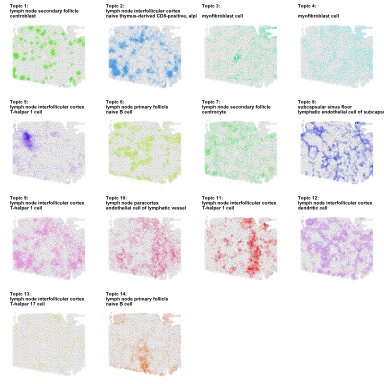
If such a data-driven approach had not yielded any confident cell-type annotations (so our deconvolved cell type gene expression profiles do not correspond to any known biological domain expert curated cell types), then we may need to go back to the drawing board and re-evaluate our underlying model assumptions and analysis approach.
Here, we do find that our deconvolved cell types’ gene expression profiles are significantly enriched for gene biomarkers of various cell types from the ASCT+B table. For example, deconvolved cell types 1’s gene expression profile is significantly enriched for gene biomarkers of centroblasts.
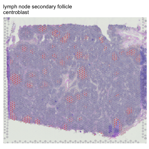
We can further visualize the deconvolved proportion of centroblasts across pixels overlaid on top of the pathology image to see that pixels where centroblasts are predicted to be highly enriched appear to correspond to the germinal center, where centroblasts are indeed expected to be!
## read histology image as rgb
img <- png::readPNG('human-lymph-node-1-standard-1-1-0/spatial/tissue_lowres_image.png')
## remove transparency
rgb <- img[,,1:3]
## make brighter
rgb <- rgb + (1-max(rgb))

## from human-lymph-node-1-standard-1-1-0/spatial/scalefactors_json.json
scalefactor <- 0.051033426
## seems like this image or coordinates may have been rotated
## crop image to same region
imagebound <- round(apply(pos2*scalefactor, 2, range))
## need some tinkering
paddingx <- 25
paddingy <- 25
imagebound[1,1] <- imagebound[1,1] - paddingx
imagebound[2,1] <- imagebound[2,1] + paddingx
imagebound[1,2] <- imagebound[1,2] - paddingy
imagebound[2,2] <- imagebound[2,2] + paddingy
shiftx <- 0
shifty <- 15
imagebound[,1] <- imagebound[,1] + shiftx
imagebound[,2] <- imagebound[,2] + shifty
print(imagebound)
rgbsub <- rgb[
    imagebound[1,2]:imagebound[2,2],
    imagebound[1,1]:imagebound[2,1],
    1:3]

## focus on just deconvolved cell type 1
## set rest to transparent
m <- deconProp[,i]
other <- 1 - m
m <- cbind(m, other)
vizAllTopics(theta = m,
             pos = pos2,
             topicCols=c("red", rgb(0,0,0,0)),
             r = 50,
             lwd = 0.1,
             showLegend = FALSE,
             overlay = rgbsub,
             plotTitle = celltype_annotations$predictions[i])
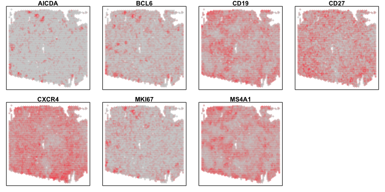
Evaluating cell type predictions
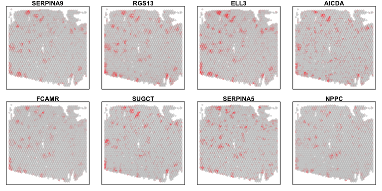
Beyond referencing the pathology image, we can also evaluate our cell type predictions by looking at the spatial patterns of the gene biomarkers. Let’s look at the gene biomarkers for centroblasts that were used in the ASCT+B tables to annotate our deconvolved cell types. Indeed, these gene biomarkers appear highly expressed at the pixels and general spatial locations where our deconvolved cell type 1 are the most abundant.
i = 1
ct <- celltype_annotations$predictions[i]
genes <- asctblist2[[ct]]
genes <- intersect(genes, rownames(gexp))

par(mfrow=c(2,4), mar=rep(1,4))
invisible(sapply(genes, function(g) {
  MERINGUE::plotEmbedding(pos2, col=gexp[g,rownames(pos2)], main=g)
}))
Further, we can dig into the inferred gene expression profiles for our deconvolved cell types. Specifically, we can see what genes are highly expressed for each of our deconvolved cell types’ gene expression profiles. Furthermore, we can see which genes are the most highly upregulated based on a log2 fold change comparison to the other deconvolved cell types’ gene expression profiles. Referencing the primary scientific literature to learn more about these genes can also help us interpret our deconvolved cell types.
## restrict to highly expressed (higher than average as arbitrary cutoff)
highexpgenes <- names(which(deconGexp[i,] > mean(deconGexp)))
## highest fold change (just take top 8)
topgenes <- names(sort(log2(deconGexp[i,highexpgenes]/
                              deconGexp[-i,highexpgenes]),
                 decreasing=TRUE))[1:8]
## plot
par(mfrow=c(2,4), mar=rep(1,4))
invisible(sapply(topgenes, function(g) {
  MERINGUE::plotEmbedding(pos2, col=gexp[g,rownames(pos2)], main=g)
}))
In this manner, we have taken a data-driven approach to make a first pass at annotating our STdeconvolve cell types using biological domain expert curated genesets from ASCT+B tables!
Try it out for yourself!
- Evaluate the cell type prediction for another deconvolved cell type.
- What happens if you try to annotate deconvolved cell types using a different ASCT+B table from the wrong tissue? What do you hypothesize should happen?
- There are many public multi-cellular pixel-resolution spatially resolved transcriptomics datasets available. Try out deconvolution analysis and annotation using ASCT+B Tables on your own.
Additional resources
STdeconvolvetutorials: https://jef.works/STdeconvolve/STdeconvolveon Github: https://github.com/JEFworks-Lab/STdeconvolveSTdeconvolveon Bioconductor: https://bioconductor.org/packages/devel/bioc/html/STdeconvolve.html
Recent Posts
- AI-guided data visualization of gas prices in different geographical locations across the US over time on 04 May 2026
- The Mentorship Index on 01 March 2026
- Vibe coding with SEraster and STcompare to compare spatial transcriptomics technologies on 22 February 2026
- RNA velocity in situ infers gene expression dynamics using spatial transcriptomics data on 13 October 2025
- Analyzing ICE Arrest Data - Part 2 on 27 September 2025