A tale of two cell populations: integrating RNA velocity information in single cell transcriptomic data visualization with VeloViz

Introduction

We recently developed a single-cell transcriptomic data visualization method called VeloViz now published in Oxford Bioinformatics. In addition to using each cell’s observed transcriptional state from single-cell transcriptomic data, VeloViz also integrates information regarding each cell’s predicted future transcriptional state inferred from RNA velocity analysis to create 2D and 3D embeddings of the data. More details regarding how the method works and its applications can be found in this paper in the journal Bioinformatics. VeloViz is implemented as an R software package avaialble at https://jef.works/veloviz/ and on Bioconductor.

In this blog post, I will use simulations to tell a story about two cell populations, who (transcriptionally) look quite similar to each other but are going in different paths (towards divergent terminal cell fates). I hope this story will be a fun demonstration of the potential utility of integrating RNA velocity information in visualizing cell populations and their relationships.

Background and Theory

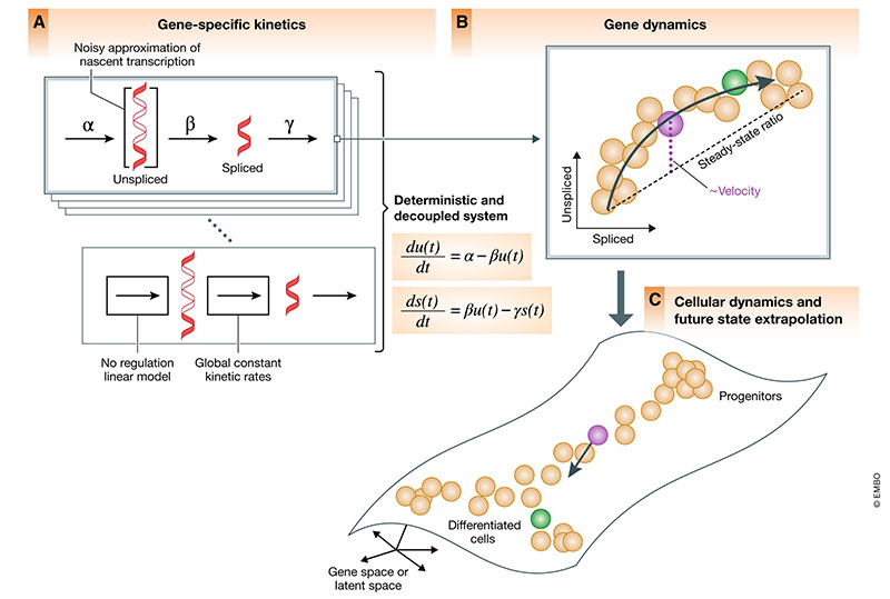
RNA velocity analysis uses the relative abundance of nascent (unspliced) and mature (spliced) mRNA to estimate the rates of gene splicing and degradation in order to predict the future transcriptional state of individual cells. In RNA velocity modeling, cells with levels of unspliced transcripts higher than expected in steady state are interpreted as having positive velocity or upregulation of the gene, while cells with levels of unspliced transcripts lower than expected at steady state are interpreted as having negative velocity or downregulation of the gene. This combination of velocities across all modeled genes can then used to estimate the future transcriptional state of each individual cell. Such RNA velocity analysis has also been adapted for transcriptomic imaging data using the relative abundance of nuclear and cytoplasmic mRNA.

Generally, in order to visualize these predicted future transcriptional states inferred from RNA velocity analysis, visualization with principal components, t-distributed stochastic neighbor embedding, and other embeddings derived from the observed transcriptional states are often used. In the rest of this blog post, I will use a very crude simulation to demonstrate the potential utility of integrating the predicted future transcriptional state information from RNA velocity in deriving embeddings for visualization purposes using VeloViz.

A tale of two cell populations (a simulation)

Let’s simulate some steady state cells and two intermediate cell populations. We will simulate two steady state cell populations (A and B) as well as two intermediate cell populations (SA and SB). In our simulation, steady state cell populations A and B have distinct transcriptional profiles. In contrast, intermediate cell populations SA and SB will express genes found in both A and B. However, we will (crudely) simulate such that SA cells are actively upregulating genes expressed in A, while SB cells are actively upregulating genes expressed in B following the theory behind RNA velocity. In particular, both SA and SB will have comparable levels of spliced RNAs but SA will have more unspliced RNAs for genes expressed in A while SB will have more unspliced RNAs for genes expressed in B.

nc <- 100
ncss <- 50

## spliced (same)
g1s <- c(rep(10,nc), rep(10,nc))
## unspliced (one high, one low)
g1us <- c(rep(15,nc), rep(5,nc))

## simulate steady state cells
ssg1s <- c(rep(0, ncss), rep(20, ncss))
ssg1us <- c(rep(0, ncss), rep(20, ncss))

## simulated ground truth expression
gts <- c(g1s, ssg1s)
gtus <-  c(g1us, ssg1us)

## group annotations
com <- c(rep('SA', nc), rep('SB', nc), rep('B', ncss), rep('A', ncss))
cell.colors <- MERINGUE:::fac2col(com)
names(gts) <- names(gtus) <- names(com) <- names(cell.colors) <-  paste0('cell', 1:c(2*nc+2*ncss))

## plot
veloviz::plotEmbedding(cbind(gts, gtus), groups=com, cex=3, 
                       xlab='Spliced', ylab='Unspliced', mark.clusters=TRUE)

## using provided groups as a factor

We can add some noise to the simulated data. Let’s also expand to 6 genes with the same upregulation trends as described previously. Note that if we were to only look at the spliced gene expression levels, SA and SB cells are transcriptionally indistinguishable. If we look at the total gene expression levels, SA, SB, A, and B cells are be distinct.

## add some noise
jitteramount <- 1
## make gene expression matrix with 6 genes
## where genes are upregulated in one of the intermediate populations
## to be more or less like the steady state populations (3 each)
spliced = rbind(jitter(c(g1s, ssg1s), jitteramount),
                jitter(c(g1s, ssg1s), jitteramount),
                jitter(c(g1s, ssg1s), jitteramount),
                jitter(20-c(g1s, ssg1s), jitteramount),
                jitter(20-c(g1s, ssg1s), jitteramount),
                jitter(20-c(g1s, ssg1s), jitteramount))
colnames(spliced) <- paste0('cell', 1:ncol(spliced))
rownames(spliced) <- paste0('gene', 1:nrow(spliced))
unspliced = rbind(jitter(c(g1us, ssg1us), jitteramount),
                jitter(c(g1us, ssg1us), jitteramount),
                jitter(c(g1us, ssg1us), jitteramount),
                jitter(20-c(g1us, ssg1us), jitteramount),
                jitter(20-c(g1us, ssg1us), jitteramount),
                jitter(20-c(g1us, ssg1us), jitteramount))

spliced[spliced < 0] <- 0
unspliced[unspliced < 0] <- 0
mat <- spliced + unspliced
colnames(unspliced) <- paste0('cell', 1:ncol(unspliced))
rownames(unspliced) <- paste0('gene', 1:nrow(unspliced))

## plot as heatmap
library(gplots)

## 
## Attaching package: 'gplots'

## The following object is masked from 'package:stats':
## 
##     lowess

gplots::heatmap.2(spliced, Rowv=NA, trace='none', ColSideColors = cell.colors, scale='none', col = colorRampPalette(c('blue', 'white', 'red'))(100))

## Warning in gplots::heatmap.2(spliced, Rowv = NA, trace = "none", ColSideColors =
## cell.colors, : Discrepancy: Rowv is FALSE, while dendrogram is `both'. Omitting
## row dendogram.

gplots::heatmap.2(mat, Rowv=NA, trace='none', ColSideColors = cell.colors, scale='none', col = colorRampPalette(c('blue', 'white', 'red'))(100))

## Warning in gplots::heatmap.2(mat, Rowv = NA, trace = "none", ColSideColors =
## cell.colors, : Discrepancy: Rowv is FALSE, while dendrogram is `both'. Omitting
## row dendogram.

Another way of looking at this is that if we were to create an UMAP embedding on the spliced gene expression levels, SA and SB cells would be intermixed. Alternatively, if we were to create an UMAP embedding on the total gene expression levels, all 4 cell populations would form distinct clusters.

set.seed(1)
emb.umap.spliced <- uwot::umap(t(spliced), min_dist = 1, n_neighbors = 5)
rownames(emb.umap.spliced) <- colnames(spliced)

par(mfrow=c(1,1))
veloviz::plotEmbedding(emb.umap.spliced, groups=com)

## using provided groups as a factor

set.seed(1)
emb.umap <- uwot::umap(t(mat), min_dist = 1, n_neighbors = 5)
rownames(emb.umap) <- colnames(spliced)

par(mfrow=c(1,1))
veloviz::plotEmbedding(emb.umap, groups=com)

## using provided groups as a factor

We can apply RNA velocity analysis to now predict the future transcriptional states of our cells. Indeed, as simulated, gene1, which is expressed in A cells but not B cells, is being upregulated in SA cells and downregulated in SB cells while gene4, which is expressed in B cells but not A cells, is being upregulated in SB cells and downregulated in SA cells.

library(velocyto.R)

## Loading required package: Matrix

cell.dist = dist(t(mat))

library(velocyto.R)
vel = velocyto.R::gene.relative.velocity.estimates(spliced, unspliced, mult=1,
                                       kCells = 10,
                                       cell.dist = cell.dist)

## calculating cell knn ... done
## calculating convolved matrices ... done
## fitting gamma coefficients ... done. succesfful fit for 6 genes
## calculating RNA velocity shift ... done
## calculating extrapolated cell state ... done

## show gene trend
emb.test <- cbind(spliced[1,], unspliced[1,])
gene <- "gene1"
velocyto.R::gene.relative.velocity.estimates(spliced, unspliced,
                                 deltaT=100,
                                 kCells = 10,
                                 kGenes=1,
                                 fit.quantile=0.1,
                                 cell.emb=emb.test,
                                 cell.colors=cell.colors,
                                 cell.dist=cell.dist,
                                 show.gene=gene,
                                 old.fit=vel,do.par=T)

## calculating convolved matrices ... done

## [1] 1

gene <- "gene4"
velocyto.R::gene.relative.velocity.estimates(spliced, unspliced,
                                 deltaT=100,
                                 kCells = 10,
                                 kGenes=1,
                                 fit.quantile=0.1,
                                 cell.emb=emb.test,
                                 cell.colors=cell.colors,
                                 cell.dist=cell.dist,
                                 show.gene=gene,
                                 old.fit=vel,do.par=T)

## calculating convolved matrices ... done

## [1] 1

Therefore, at a future time point, we would expect the expression level of gene1 in SA cells to be higher, like that in A cells, while the expression level of gene1 in SB cells to be lower, like that in B cells. Likewise, we would expect the expression level of gene4 in SA cells to be lower, like that in A cells, while the expression level of gene4 in SB cells to be higher, like that in B cells.

curr = vel$current
proj = vel$projected

par(mfrow=c(1,2))
veloviz::plotEmbedding(cbind(mat[1,], curr[1,]), groups=com,
                       xlab='Observed Total', ylab='Current Spliced', mark.clusters=TRUE)

## using provided groups as a factor

veloviz::plotEmbedding(cbind(mat[1,], proj[1,]), groups=com, 
                       xlab='Observed Total', ylab='Projected Spliced', mark.clusters=TRUE)

## using provided groups as a factor

VeloViz can take into consideration this predicted future transcriptional state in creating the embedding and visualizing these cell populations. By taking into consideration the predicted future transcriptional states, we can see more clearly see in the VeloViz embedding that SA cells are closer to A cells while SB cells are closer to B cells.

library(veloviz)
# build VeloViz graph
veloviz = veloviz::buildVeloviz(
  curr = curr, proj = proj,
  normalize.depth = FALSE,
  use.ods.genes = FALSE,
  pca = FALSE,
  k = 5,
  similarity.threshold = 0,
  distance.weight = 1,
  distance.threshold = 0,
  weighted = TRUE,
  seed = 0,
  verbose = FALSE
)

## [1] "Done finding neighbors"
## [1] "calculating weights"
## [1] "Done making graph"

emb.veloviz = veloviz$fdg_coords

par(mfrow=c(1,1))
veloviz::plotEmbedding(emb.veloviz, groups=com, mark.clusters = TRUE)

## using provided groups as a factor

We can further visualize RNA velocity arrows on each of these embeddings to get a sense for how these 4 cell populations (SA, SB, A, and B) may be related to each other.

par(mfrow=c(1,1))
show.velocity.on.embedding.cor(scale(emb.umap.spliced), vel,n=100,scale='sqrt',cell.colors=cell.colors, arrow.scale = 0.5, arrow.lwd=1, do.par = FALSE, show.grid.flow=TRUE,min.grid.cell.mass=0.5,grid.n=20)

## delta projections ... sqrt knn ... transition probs ... done
## calculating arrows ... done
## grid estimates ... grid.sd= 0.1621915  min.arrow.size= 0.00324383  max.grid.arrow.length= 0.08212338  done

show.velocity.on.embedding.cor(scale(emb.umap), vel,n=100,scale='sqrt',cell.colors=cell.colors, arrow.scale = 0.5, arrow.lwd=1, do.par = FALSE, show.grid.flow=TRUE,min.grid.cell.mass=0.5,grid.n=20)

## delta projections ... sqrt knn ... transition probs ... done
## calculating arrows ... done
## grid estimates ... grid.sd= 0.1348527  min.arrow.size= 0.002697054  max.grid.arrow.length= 0.08212338  done

show.velocity.on.embedding.cor(scale(emb.veloviz), vel,n=100,scale='sqrt',cell.colors=cell.colors, arrow.scale = 0.5, arrow.lwd=1, do.par = FALSE, show.grid.flow=TRUE,min.grid.cell.mass=0.5,grid.n=20)

## delta projections ... sqrt knn ... transition probs ... done
## calculating arrows ... done
## grid estimates ... grid.sd= 0.146899  min.arrow.size= 0.002937981  max.grid.arrow.length= 0.08212338  done

Indeed, by taking into consideration the predicted future transcriptional states, we can see more clearly see in the VeloViz embedding that SA cells are transcriptionally moving towards A cells while SB cells are transcriptionally moving towards B cells. In contrast, UMAP embeddings that take into consideration only the observed spliced or total gene expression levels are not able to preserve such transcriptional relationships between populations.

Of course, this is a very crude and simple simulation highlighting the theoretical utility of taking into consideration information from RNA velocity information in visualizing cellular trajectories. Try it out for yourself! Can you simulate a scenario where taking into consideration RNA velocity information in visualizing cellular trajectories better recapitulates the underlying expected cell population relationships? What about a scenario where taking into consideration RNA velocity information misleads by suggesting a relationship between cell populations that should not exist? Are there instances with real data where these scenarios may apply? What orthogonal evidence and experiments can you do to follow up?

Additional Resources

• VeloViz paper in Oxford Bioinformatics
• VeloViz software and tutorials
• Original RNA velocity paper
• Dynamic RNA velocity paper
• Alternative RNA velocity in situ for imaging data paper
• Review of RNA velocity - current challnges and future perspectives